Helmholtz Resonance (Plenum Pressure Model)
Case directory
$FOAM_TUTORIALS/compressible/rhoPimpleFoam/laminar/helmholtzResonance
Summary
We calculate air flow in a channel with a narrowed center, and see the pressure oscillation due to Helmholtz resonance.
The region "plenum" is modeled using the boundary condition type "plenumPressure" to reduce the calculation amount by omitting the upstream part of the channel. The fluid flows out of the region "outlet". The region "walls" is set to be a stationary wall with zero velocity and the region "symmetry" is set to a symmetric boundary.
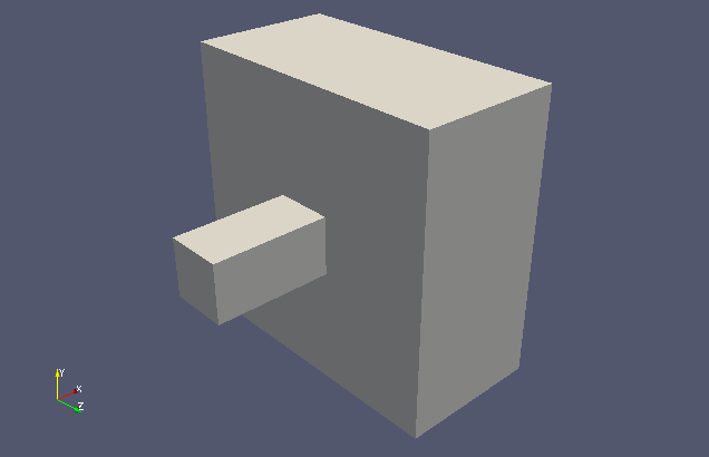 Model geometry
 Summary for model geometry
The boundary condition type "plenumPressure" is defined in the file modelled/0/p as follows. The boundary condition type "plenumPressure" can be used to simulate the plenum pressure at the inlet.
plenum
{
	type            plenumPressure;
	gamma           1.4;
	R               287.04;
	supplyMassFlowRate 0.0001;
	supplyTotalTemperature 300;
	plenumVolume    0.000125;
	plenumDensity   1.1613;
	plenumTemperature 300;
	inletAreaRatio  1.0;
	inletDischargeCoefficient 0.8;
	timeScale       1e-4;
	value           uniform 1e5;
}
And, the following settings are made in the file modelled/system/controlDict, and pressure sampling is performed at five locations. The sampling results are saved in the file modelled/postProcessing/probes/0/p.
functions
{
	probes
	{
		libs ( "libsampling.so" );
		type probes;
		name probes;
		writeControl timeStep;
		writeInterval 1;
		fields ( p );
		probeLocations
		(
			( -0.045  0     0)
			( -0.045  0.020 0)
			( -0.010  0     0)
			(  0.0125 0     0)
			(  0.0125 0.020 0)
		);
	}
}
The meshes are as follows, and the number of mesh is 13632.
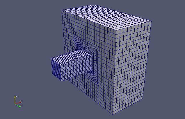 Meshes
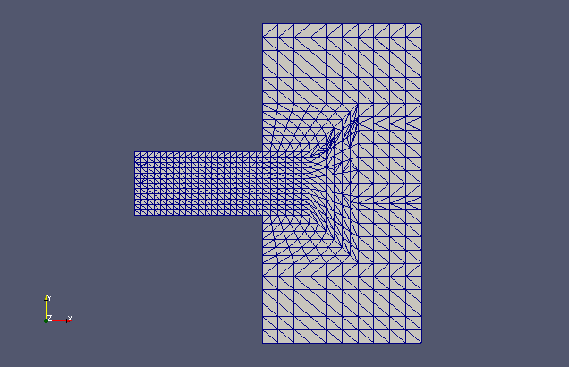 Meshes (XY-plane)
The calculation result is as follows.
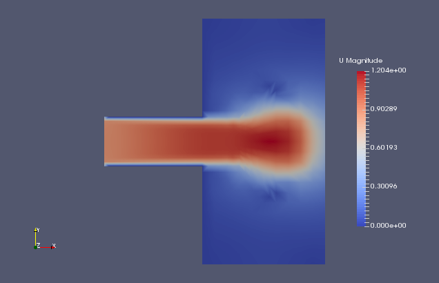 Flow velocity at final time (U)
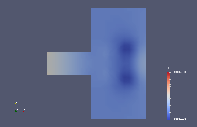 Pressure at final time (p)
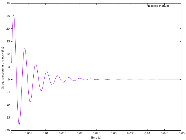 Time series of pressure at sampling point (-0.01, 0, 0) (p)
 Position of sampling point (-0.01, 0, 0)
A comparison of the pressures at the sampling points (-0.01, 0, 0) with the case where the plenum pressure is not modeled but calculated over the entire field including the upstream part (tutorial "Helmholtz Resonance") is shown below.
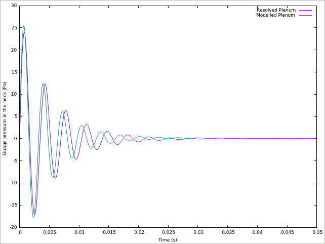 Comparison of entire field calculation (Resolved Plenum: magenta) and modeled calculation (Modelled Plenum: cyan)
Commands
cd helmholtzResonance
# Required to use the command "cloneCase"
. $WM_PROJECT_DIR/bin/tools/RunFunctions
# Create a case from the template file
cd system
ln -s blockMeshDict.modelledBlocks blockMeshDict.caseBlocks
ln -s blockMeshDict.modelledBoundary blockMeshDict.caseBoundary
cd ../
cloneCase . modelled
# Calculate the case we created
cd modelled
blockMesh
decomposePar
mpirun -np 4 rhoPimpleFoam -parallel
reconstructPar
paraFoam
# Plot the time variation of pressure, with the first column as the horizontal axis and the fourth column minus 100000 as the vertical axis.
gnuplot
gnuplot> set xlabel "Time (s)"
gnuplot> set ylabel "Guage pressure in the neck (Pa)"
gnuplot> plot "postProcessing/probes/0/p" using 1:($4-1e5) title "Modelled Plenum" with lines
Calculation time
9.48 seconds *4 parallel, Inter(R) Core(TM) i7-8700 CPU @ 3.20GHz 3.19GHz
Reference
- Helmholtz resonance - Wikipedia
- OpenFOAM-4.x/src/finiteVolume/fields/fvPatchFields/derived/plenumPressure/plenumPressureFvPatchScalarField.H - GitHub