Tutorial : Measuring drag coefficient on simple car model

Updated: October 8, 2022

In this tutorial, we will create analysis area around a imporing shape and setting files for OpenFOAM^® and output force coefficient values such as drag coefficient and lift coefficient.

Table of Contents

Analysis summary
Creating an analysis configuration file
Running a calculation
Confirming a calculation result
References

Analysis summary

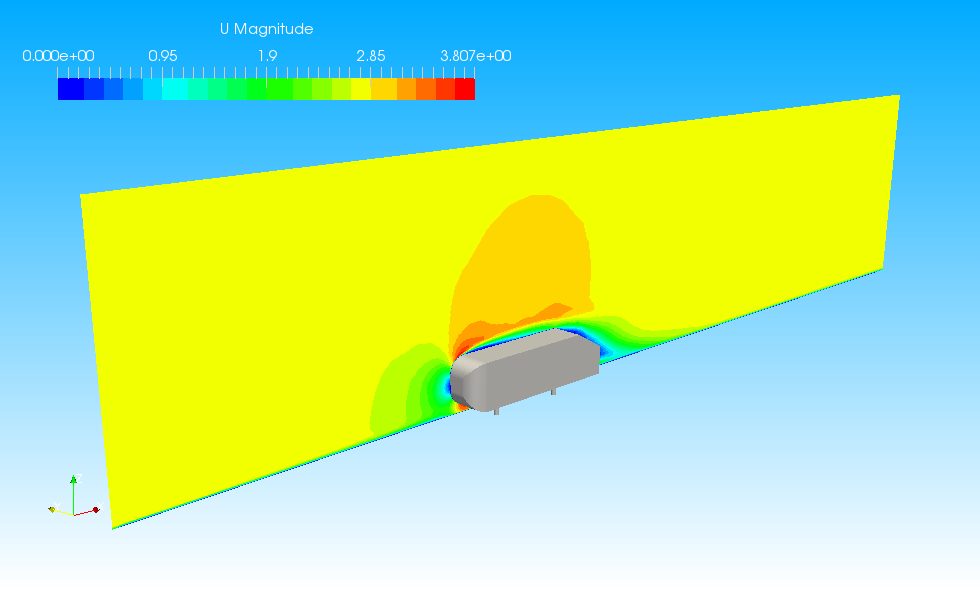
We will calculate the external flow around a simple car-model (Ahmed body) for 5 seconds in simulation time. The model is placed in a air flow of approximately 10 km/h. And we will set the output settings to obtain the values of drag coefficient, lift coefficient and others at each time.

ParaFoam velocity result — Analysis result

Creating an analysis configuration file

Creating a project

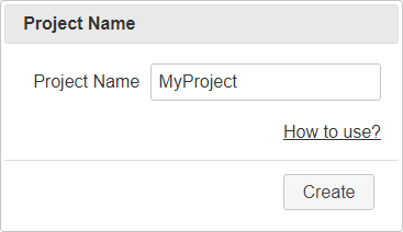
Open XSim. Type "MyProject" as Project Name and click Create button to create project.

Importing shapes

We will use a prepared shape file in this tutorial. Please download a zipped file from next link, "tutorial-AhmedBody.zip", and extract it.

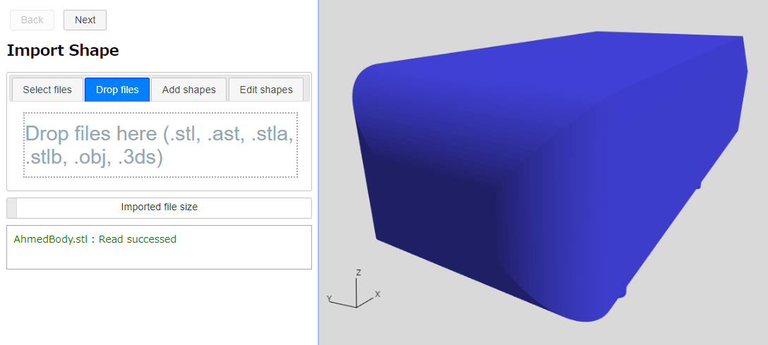
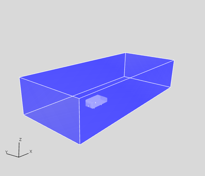
Drag&Drop the extracted file "AhmedBody.stl" at "Drop files" tab and load it. The loaded shape will be shown in 3D view.

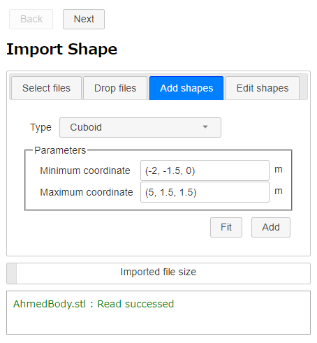
Select "Cuboid" as type in "Add shapes" tab and set (-2, -1.5, 0) m to minimum coordinate, (5, 1.5, 1.5) m to maximum coordinate. Then click Add. You can switch the 3D display to semitransparent by clicking a display-mode buttonunder 3D view.

Adding a shape for analysis area (3D view)

Note: Size of Analysis Area for External Flow

In the analysis of external flow, it is desirable to set the analysis area as large as possible to reduce the influence of analysis area boundaries. However, a larger analysis area increases the computational cost in terms of computation time and memory usage, so an appropriate balance will be required.

As shown in the following figure, it is known empirically that the influence of the boundary can be reduced by setting a distance of 2L upstream, 5~10L downstream, and 5L in the lateral direction, where L is the maximum length of the analysis target.

The blockage ratio, which is the ratio of the frontal projected area of the analysis target to the cross-sectional area of the analysis area, may be used as a criteria for the lateral distance. When the blockage ratio is used as a standard, it should be less than 100% to 60% for environmental wind tunnels and less than 10% for aerodynamic wind tunnels used to measure force characteristics (References [1][2][3]).

Click Next button to go to Mesh page.

Mesh

Refinement settings

Select "Cuboid" as range type in "Refinement settings" and set (-0.1, -0.5, 0) m to minimum coordinate, (3, 0.5, 0.5) m to Maximum coordinate. And set 2 to refinement level. Preview the range shape by clicking preview button, then click Add.

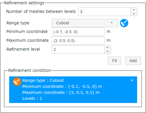
Refinement settings (Cuboid)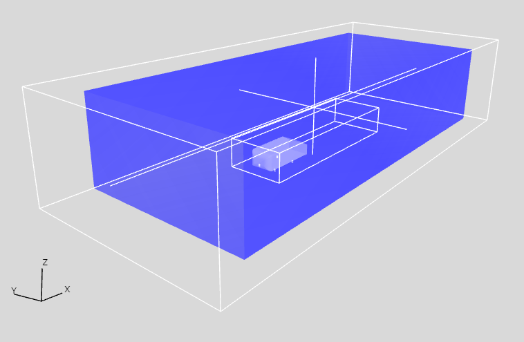

Cuboid area for refinement

Then select "Surface (Region)" as range type in "Refinement settings" and "AhmedBody" as region. Set 3 to refinement level and click Add.

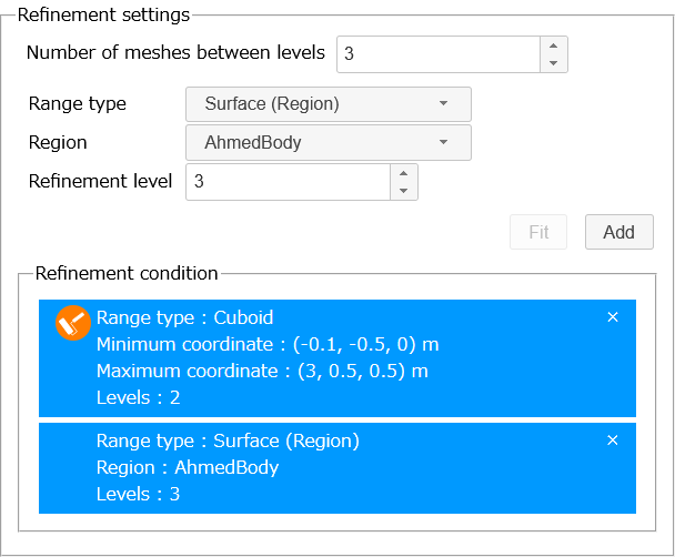
Refinement settings (Surface)
Layer mesh settings

Confirm that 0.3 is set to layer thickness ratio and 3 is set to number of layers. Click "AhmedBody" and "ZMin" in Navigation view at left side of the window to select, then click Set.

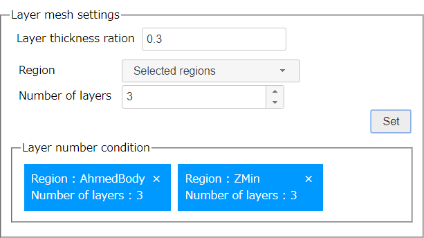
Layer mesh settings

Click Next button to go to Basic Settings page.

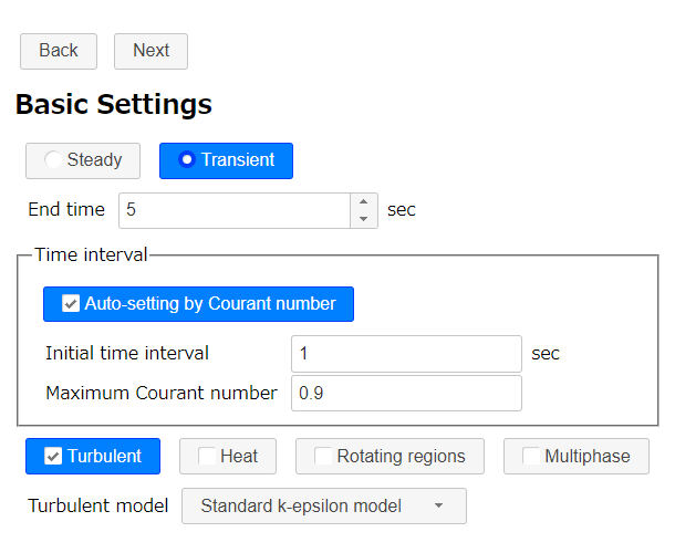
Basic Settings

In this section, we will set a type of analysis. Select "Transient" and set 5 seconds as end time.

Click Next button to go to Physical Property page.

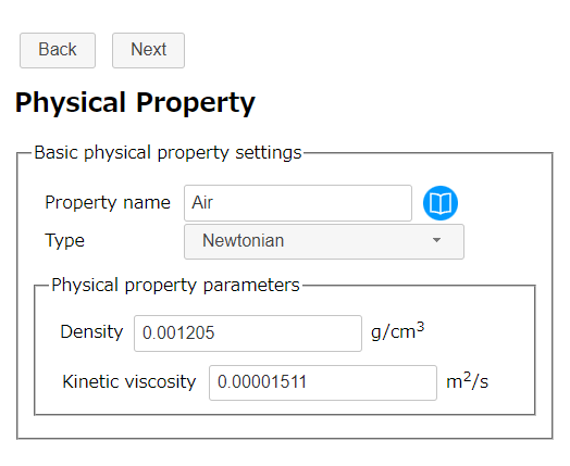
Physical Property

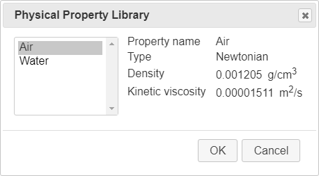
In this section, we will set a type of fluid. Click Physical property library buttonto show dialog. Select "Air" in the dialog and click OK.

Click Next button to go to Initial Condition page.

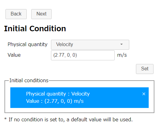
Initial Condition

We will set initial flow field to get final solution as early as possible. Select "Velocity" as physical quantity and set (2.77, 0, 0) m/s as value. Then click Set.

Click Next button to go to Flow Boundary Condition page.

Flow Boundary Condition

Inflow boundary

Select "Selected regions" as region and "Fixed flow velocity" as type. Then select "XMin" on Navigation view and set (2.77, 0, 0) m/s as flow velocity. After that, click Set.

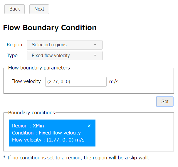
Inflow boundary condition
Outflow boundary

Select "Selected regions" as region and "Fixed static pressure" as type. Then select "XMax" on Navigation view and set 0 Pa as static pressure. After that, click Set.

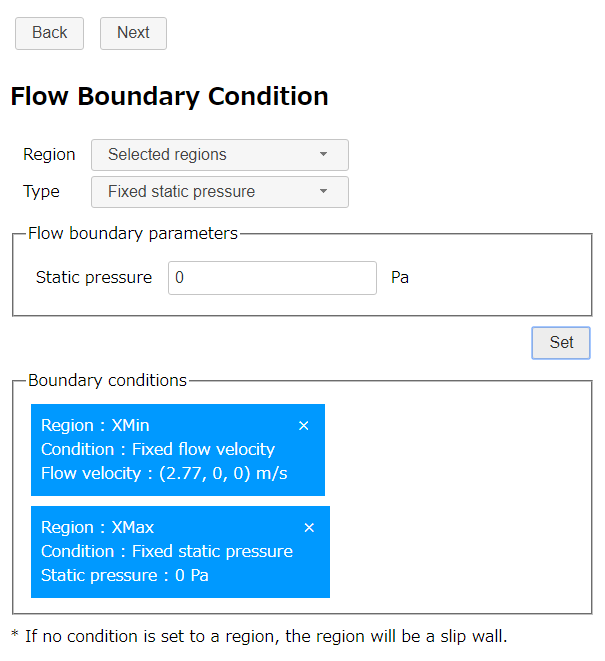
Outflow boundary condition
Stationary wall boundary

Select "Selected regions" as region and "Stationary wall" as type. Then select "AhmedBody" and "ZMin" on Navigation view and click Set.

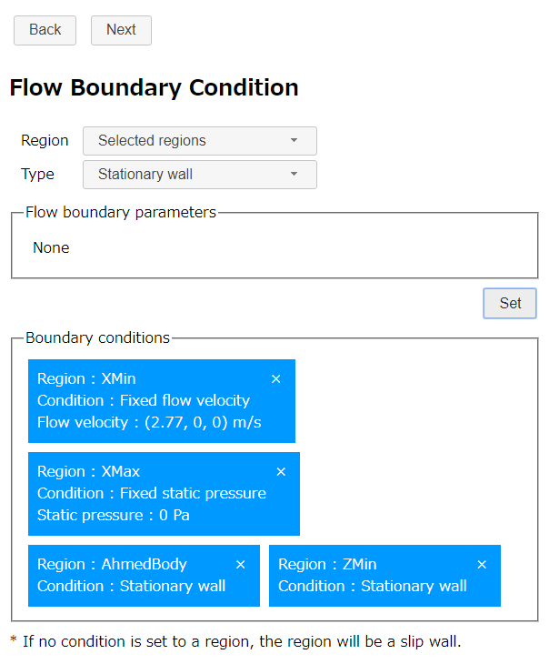
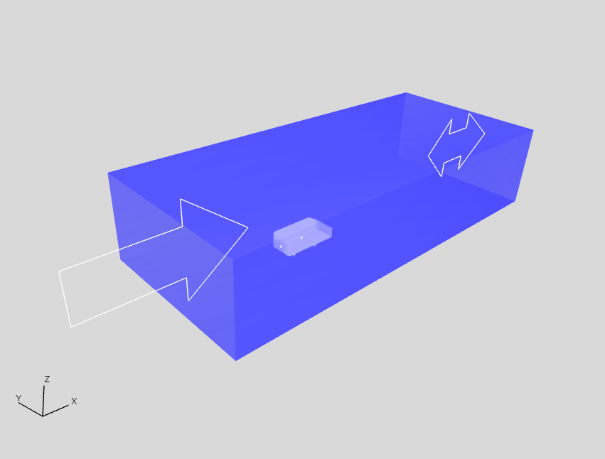
Wall boudary condition

Inflow boudary and outflow boudary are displayed as arrows in 3D view.

Inflow/Outflow boundaries will be shown in 3D view

Click Next button to go to Calculation Settings page.

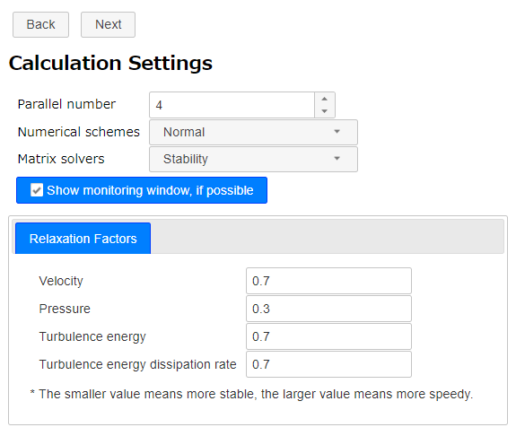
Calculation Settings

In this section, we set parallel number of CPU core that we use in this calculation (for example, 4).

Click Next button to go to Output page.

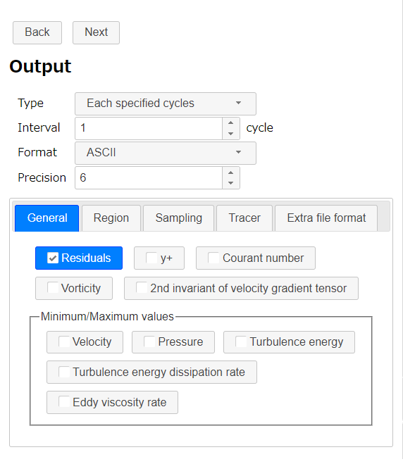
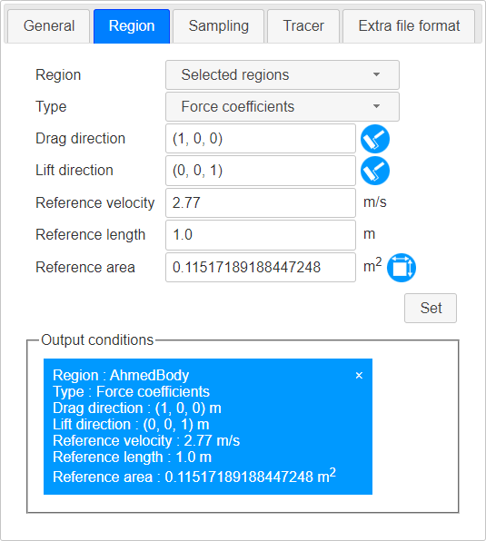
Output

Because this analysis is a transient analysis, select "Each specified time" as type and set 1 second to interval.

Next, we will set to output drag coefficient.

Select "Region" tab and select "Selected regions" as region and "Force coefficients" as type. Then set 2.77 m/s as Reference velocity.

Select "AhmedBody" on Navigation view and click Measure projection area button to show Projection Area dialog. Then click OK to set Reference area.

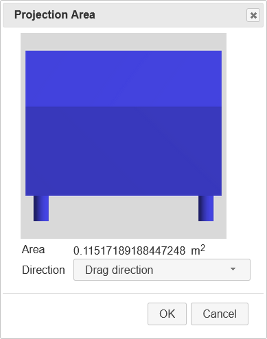
After setting all parameters, click Set button to set Force coefficients output setting.

Click Next button to go to Export page.

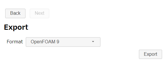
Export

Finally we finished all settings. Click Export button to export the analysis setting as zipped OpenFOAM case directory "MyProject.zip". The zip file download starts immediately.

Running calculation

Extract downloaded file "MyProject.zip". There is a bash-script "Allrun " in the case directory. So run the script to make mesh and start the OpenFOAM solver by following command.

./Allrun

If the machine that calculation is running has desktop environment and gunuplot was installed, residual convergence chart will be displayed.

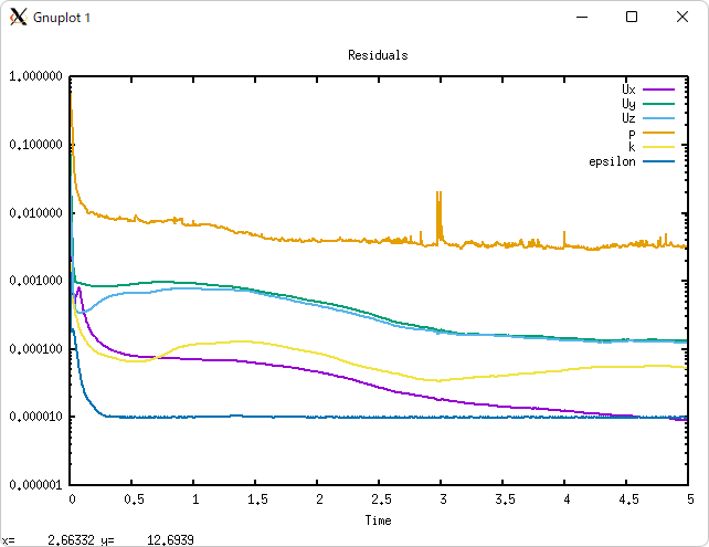
Running in 4 parallel (Inter(R) Core(TM) i7-8700 CPU @ 3.20GHz 3.19GHz), it takes 10 seconds to create a mesh and about 8 minutes to analyze.

Confirming calculation result

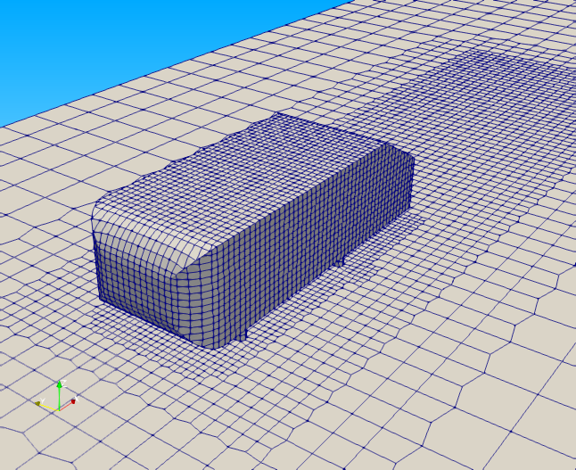
After the calculation, execute a following command to visualize the mesh and the calculation result.

paraFoam

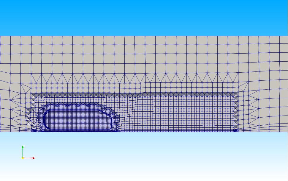
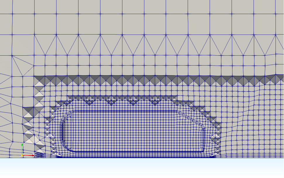
Mesh is following.

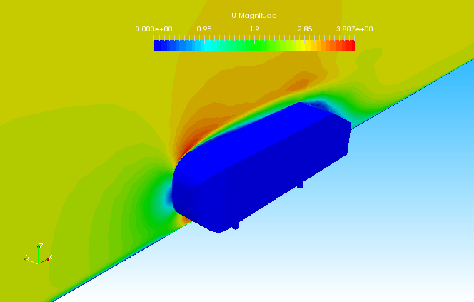
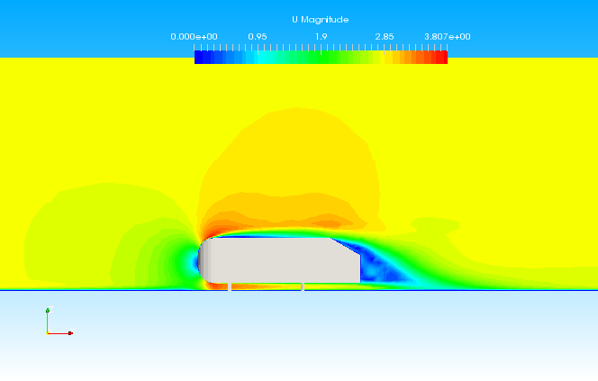
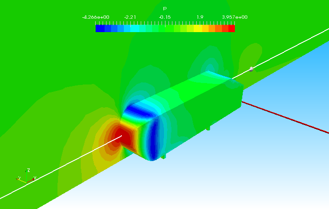
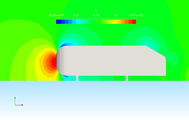
Mesh of cross section in flow direction (zoom)

Distributions of Flow velocity and pressure are following.

Flow velocity distribution (only fluid-side)

Drag coefficient and other force coefficients are output at forceCoeffs.dat file in postProcessing/forceCoeffs(AhmedBody)/0 folder as following.

# Force coefficients
# liftDir     : (0.000000e+00 0.000000e+00 1.000000e+00)
# dragDir     : (1.000000e+00 0.000000e+00 0.000000e+00)
# pitchAxis   : (0.000000e+00 -1.000000e+00 0.000000e+00)
# magUInf     : 2.770000e+00
# lRef        : 1.000000e+00
# Aref        : 1.151719e-01
# CofR        : (3.369437e-01 2.145408e-05 7.275021e-02)
# Time        	Cm            	Cd            	Cl            	Cl(f)         	Cl(r)       
0             	-5.587547e-03	7.058447e-02	5.698159e-04	-5.302639e-03	5.872454e-03
0.000361925   	-1.563391e+01	1.850193e+02	4.270235e+01	5.717266e+00	3.698508e+01
0.000783536   	-1.687351e+01	2.081231e+02	5.050325e+01	8.378113e+00	4.212514e+01
……(省略)……
4.99739       	9.405859e-02	4.975069e-01	5.129965e-01	3.505568e-01	1.624397e-01
4.9987        	9.400983e-02	4.974598e-01	5.128405e-01	3.504301e-01	1.624104e-01
5             	9.397174e-02	4.974367e-01	5.127337e-01	3.503386e-01	1.623951e-01

Cm, Cd and Cl represent the torque coefficient, drag coefficient and lift coefficient. Cl(f) and Cl(r) is defined by "Cl/2.0 + Cm" and "Cl/2.0 - Cm".

References

[1] "All Weather Testing Chamber for Automobiles", Hiroshige FUKUSAWA, koji NAKAGAWA, Masanori YOSHIDA, 1987.（Japanese, PDF）
[2] "LES on full scale vehicle model with detailed tire", Kanade TAKEUCHI, Makoto TSUBOKURA, 2015.（Japanese, PDF）
[3] "What is blockage ratio?" - CFD Online Discussion Forums