Tutorial - Calculation of axial fan with moving mesh function
In this tutorial, we will calculate a rotating axial fan with moving mesh function.
Analysis summary
We wll calculate an axial fan rotating at a speed of 120°/sec for 10 seconds. We also set the output setting to get the flow rate generated by the rotation of the axial fan.
Creating an analysis configuration file
Creating a project
Open XSim. Type "AxialFan" as Project Name and click button to create project.

Importing shapes
We will use a prepared shape file in this tutorial. Please download a zipped file from next link, "tutorial-AxialFan.zip", and extract it.
Drag&Drop the extracted files "fan.stl", "inlet.stl", "outlet.stl" and "side.stl" at "Drop files" tab and load it. The loaded shape will be shown in 3D view.
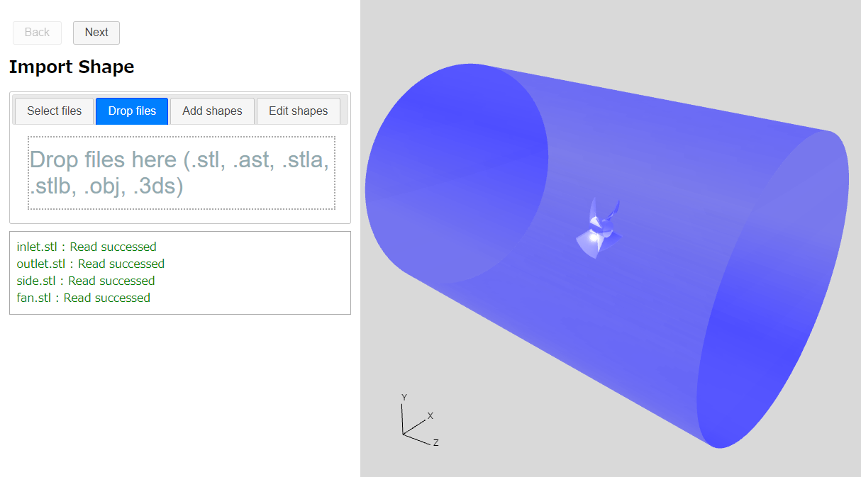
You can switch the 3D display to semitransparent by clicking a display-mode button under 3D view.
Click button to go to Mesh page.
Mesh
-
Volume mesh settings
Set 80000 as target number of base meshes and (0, 0, 0.5) as computational domain.
Note: You can not set the computational domain definition point in the rotation area. It must be set on the stationary area.
-
Refinement settings
In Refinement settings, select "Cylinder" as range type and set 0.135 m to radius, (0, 0, 0.065) m to center of top, (0, 0, -0.03) m to center of bottom. Then set 2 to refinement level. Preview the range shape by clicking preview button
 , then click .
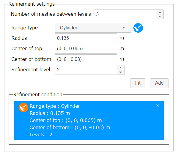
Refinement setting (Cylinder) 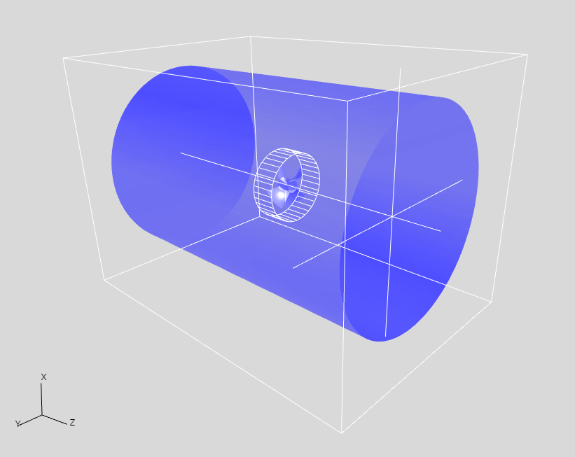
Cylindrical area for refinement -
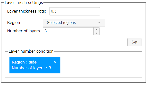
Layer mesh settings
Confirm that 0.3 is set to layer thickness ratio and 3 is set to number of layers. Click "side" in Navigation view at left side of the window to select, then click .
Layer mesh settings
Click button to go to Basic Settings page.
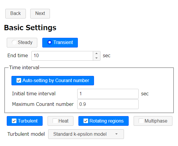
Basic Settings
In this section, we will set a type of analysis. Select "Transient" and set 10 seconds as end time. Then select "Rotating regions".
Click button to go to Physical Property page.
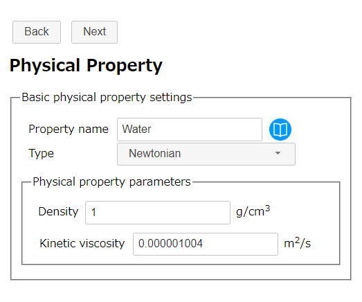
Physical Property
No configuration is required because we will use default physical property. Confirm that "Water" is set as the physical property value.
Click button to go to Initial Condition page.
Initial Condition
No configuration is required because we will use default parameters. Click button to go to Flow Boundary Condition page.
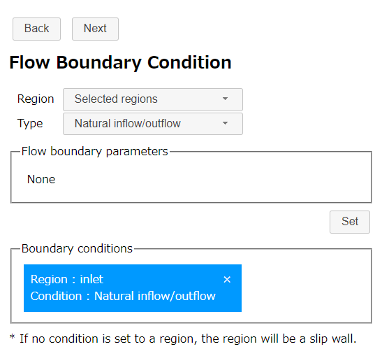
Flow Boundary Condition
-
Inflow boundary
Select "Selected regions" as region and "Natural inflow/outflow" as type. Then select "inlet" on Navigation view and click .
Inflow boundary condition -
Outflow boundary
Select "Selected regions" as region and "Fixed static pressure" as type. Then select "outlet" on Navigation view and set 0 Pa as static pressure. After that, click .
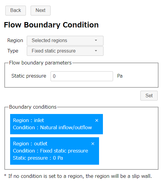
Outflow boundary condition -
Stationary wall boundary
Select "Selected regions" as region and "Stationary wall" as type. Then select "side" and "fan" on Navigation view and click .
Note: The stationary wall condition must be set for any wall that moves in rotation.
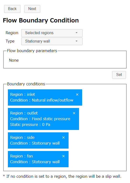
Wall boundary condition
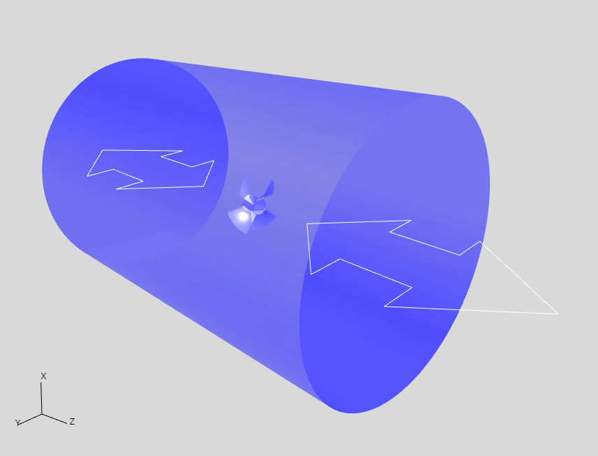
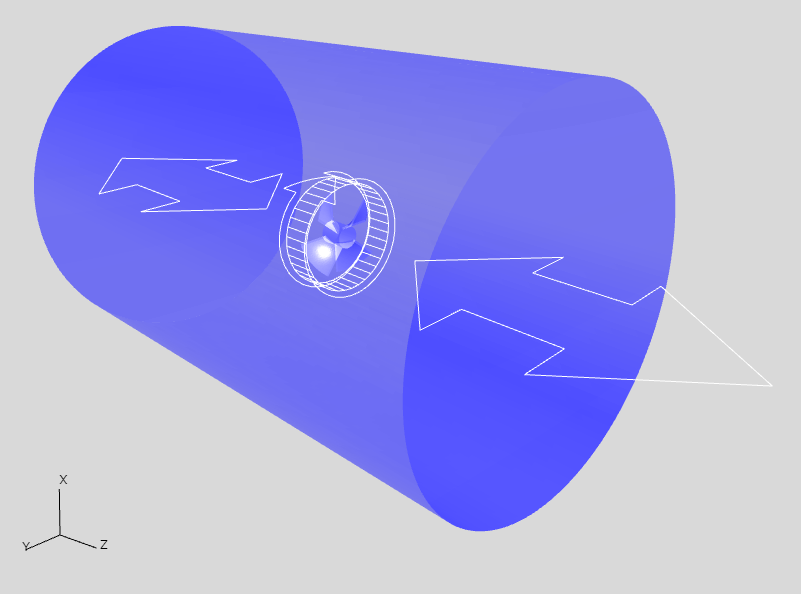
Inflow boudary and outflow boudary are displayed as arrows in 3D view.
Click button to go to Rotating Region page.
Rotating Region
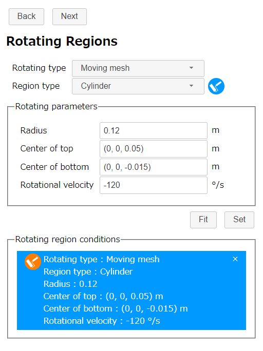
Select "Moving mesh" as rotating type and "Cylinder" as region type. Then set 0.12 m to radius, (0, 0, 0.05) m to center of top, (0, 0, -0.015) to center of bottom and -120 °/s to rotational velocity. Preview the rotating region and rotational direction by clicking preview button, then click .
You can select "MRF" or "Moving mesh" as rotating type. Each has the following advantages and disadvantages.
-
MRF
By adding the effect of rotational volume force (centrifugal force, Coriolis force) to the specified area, the rotation is simulated without rotating the shape.
Advantages: It can be used for both steady and transient analysis, and is often more stable and faster than the Moving mesh calculations.
Disadvantages: The flow must be rotational symmetry about the rotating area, otherwise (e.g. cross flow fan) the flow cannot be reproduced correctly. Also, it may be difficult to see the rotational velocity when visualizing the results because the shape does not actually rotate.
-
Moving mesh
By actually rotating the mesh in the specified area, it reproduces the rotation of the shape.
Advantages: It can be used for any flow. It is easy to see the rotation velocity when visualizing the results, because the shape actually rotates.
Disadvantages: It cannot be used for steady analysis. Also, the calculation is often more unstable and slower than the MRF because the mesh is actually moved.
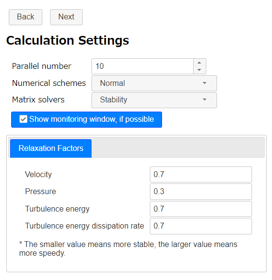
Calculation Settings
In this section, we set parallel number of CPU core that we use in this calculation (for example, 10).
Click button to go to Output page.
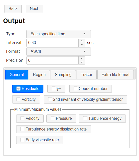
Output
Because this analysis is a transient analysis, select "Each specified time" as type and set 0.33 second to interval.
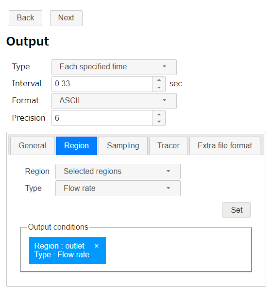
Next, set the output for the flow rate.
Select "Region" tab and set "Selected regions" as region and "Flow rate" as type. Select "outlet" on Navigation view and click .
Click button to go to Export page.
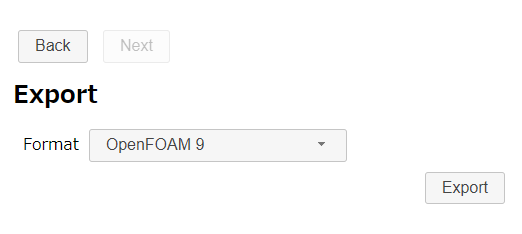
Export
Finally we finished all settings. Click button to export the analysis setting as zipped OpenFOAM case directory "AxialFan.zip". The zip file download starts immediately.
Running a calculation
Extract downloaded file "AxialFan.zip". There is a bash-script "Allrun " in the case directory. So run the script to make mesh and start the OpenFOAM solver by following command.
If the machine that calculation is running has desktop environment and gunuplot was installed, residual convergence chart will be displayed.
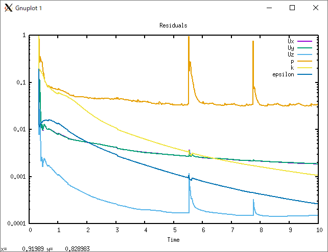
Running in 10 parallel (Inter(R) Core(TM) i7-8700 CPU @ 3.20GHz 3.19GHz), it takes 10 seconds to create a mesh and about 8 minutes to analyze.
Confirming a calculation result
After the calculation, execute a following command to visualize the mesh and the calculation result.
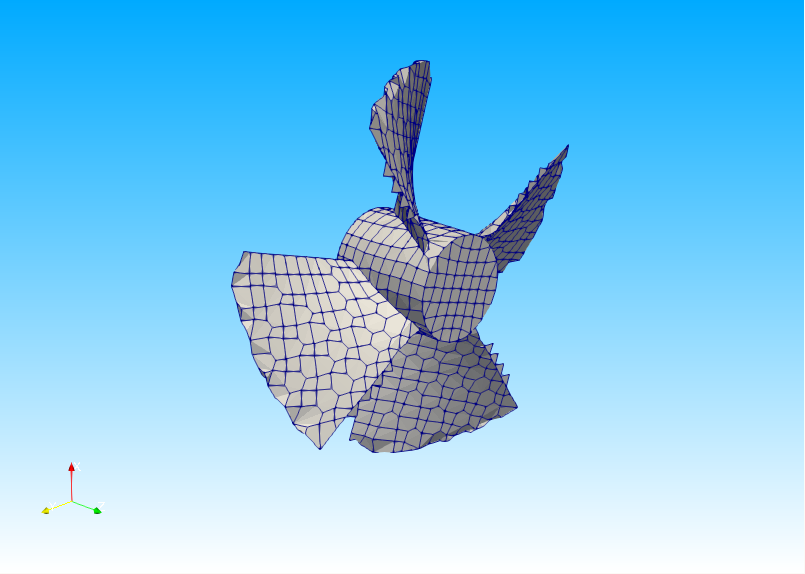
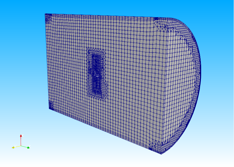
Mesh is as follows.
We used a coarse meshes to shorten the calculation time, but if you want to make the fan shape more precisely, you can make a finer mesh.
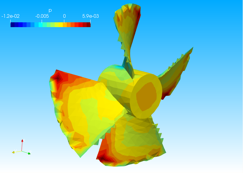
The pressure distribution at the fan surface at the final time is as follows.
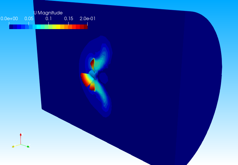
And the flow velocity has been changing as shown in the video below.
The flow rate will be outputed to the text file "surfaceFieldValue.dat" in "postProcessing/patchFlowRate(patch=outlet)/0" as following . The left side column is time and the right side column is flow rate.
# Region type : patch outlet
# Faces  :    2011
# Area   :    5.025600e-01
# Time        	sum(phi)
0             	0.000000e+00
0.66          	6.402070e-05
0.672453      	5.972452e-05
…………
9.97452       	4.939671e-04
9.98516       	4.944257e-04
9.99581       	4.948761e-04