Tutorial - Calculation of dam break problem with multiphase function
In this tutorial, we will calculate 2 liquids dam break problem with multiphase function.
Analysis summary
The dam break problem consisted of 2 liquids "Water" and "Kerosene", and we wll calculate the flow for 5 seconds.
Creating an analysis configuration file
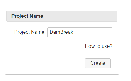
Creating a project
Open XSim. Type "DamBreak" as Project Name and click button to create project.
Importing shapes
We will make a space for the analysis at first. Select "Cuboid" as Type, then enter (0, 0, 0) as Minimum coordinate and (1, 1, 1) as Maximum coordinate. Push to add a space for the analysis. The shape of analysis region will be displayed at 3D view.
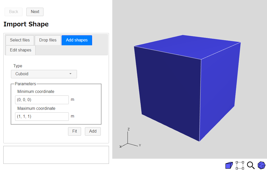
Click button to go to Mesh page.
Mesh
Enter 200000 as Target number of base meshes. The base meshes can be previewed with the preview button that next to the Number of base meshes.
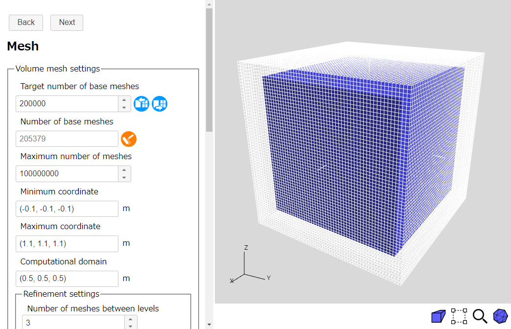
The mesh settings is over. Click button to go to Basic Settings page.
Basic Settings
We will set analysis tyoe settings. Select "Transient" and enter "5 sec" as End time. Enter "0.01 sec" as Initial time interval. Then select "Multiphase" and enter "0 Pa" as Reference pressure.
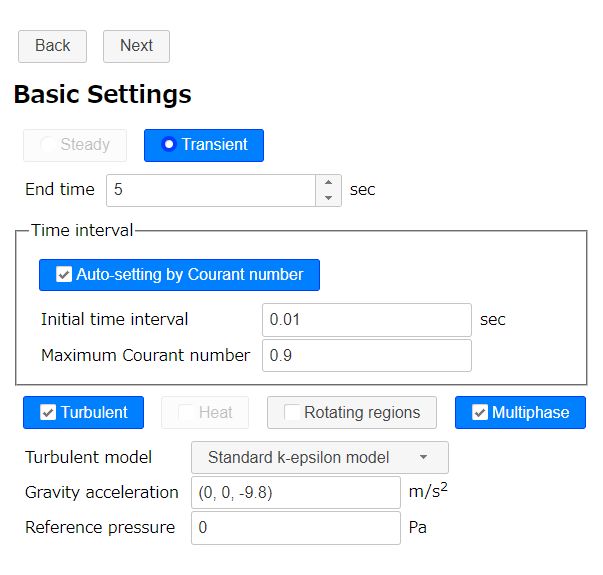
Click button to go to Physical Property page.
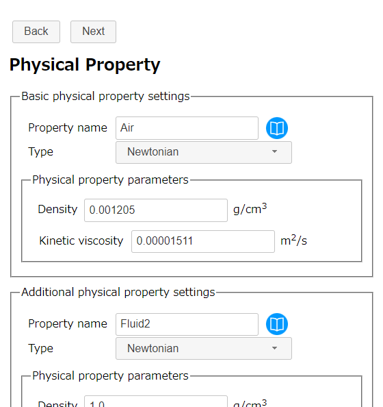
Physical Property
At first, we will set basic physical property.
We want to calculate 2 liquids flow in the space filled with air. So we will set air as basic physical property. Push library button at "Basic physical property settings" and select "Air" from the library as basic physical property.
Then we will set 2 liquids "Water" and "Kerosene" as additional physical properties.
Push library button at "Additional physical property settings" and select "Water" from the library. Then push to register the water as additional physical property.
We will make the property of kerosene manually, because it does not exist in the library. Enter "Kerosene" as Property name, "Newtonian" as Type, "0.8 g/cm3" as Density and "0.000239 m2/s" as Kinetic viscosity. Then push to register the property of kerosene.
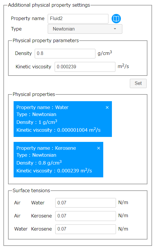
We need to set a surface tension values between each fluid, but for this tutorial we will simplify all of them to "0.07 N/m".
Click button to go to Initial Condition page.
Initial Condition
Next we will set the initial range of the 2 liquids.
Select "Fluid" as Physical quantity, "Water" as Property name and "Cuboid" as Range type. Then enter (0, 0, 0) m as Minimum coordinate and (0.4, 0.4, 0.8) m as Maximum coordinate. Push to set initial range of water.
Similarly, select "Fluid" as Physical quantity, "Kerosene" as Property name and "Sphere" as Range type. Enter (0.7, 0.7, 0.5) m as Center and 0.25 m as Radius. Then push to set initial range of kerosene.
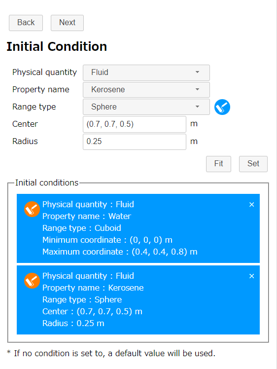
If the initial ranges overlapped, the one displayed lower in the initial condition area will take priority. For example, in the above figure, the initial range of water will be written over by the initial range of kerosene. The order of the conditions can be changed by mouse dragging.
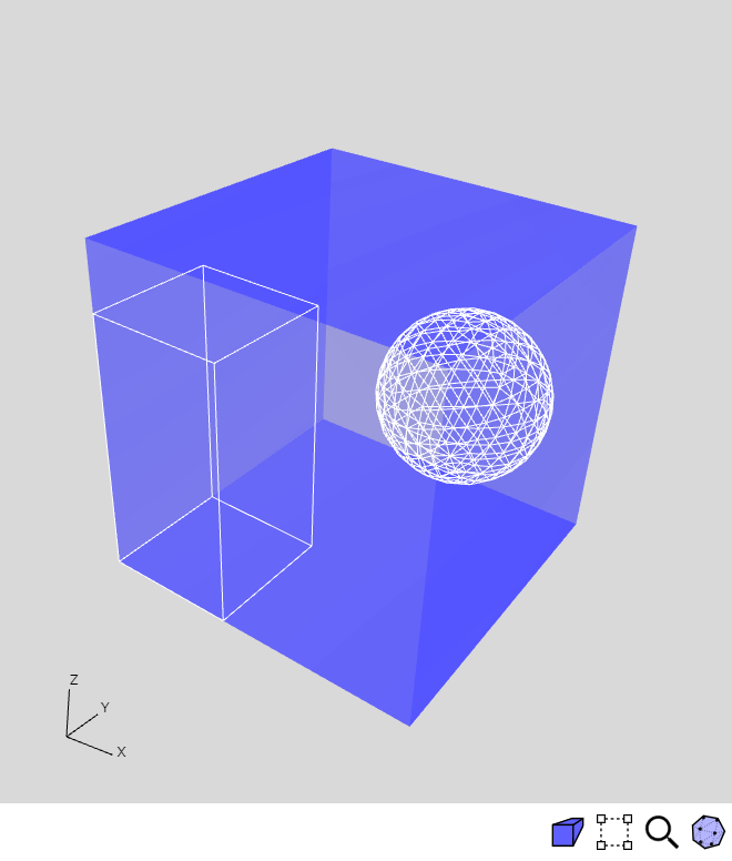
We can preview the shapes of the initial range by switch the 3D view to semi-transparent  and push the preview button for each conditions.
The initial condition settings is over. Click button to go to Flow Boundary Condition page.
Flow Boundary Condition
In this tutorial, we will assume that only the X maximum face is open, and that the other faces are stationary walls.
-
Inflow/outflow boundary
Select "Selected regions" as Region, "Natural inflow/outflow" as Type and "Air" as Inflow fluid. Then select "XMax" in navigation view and push .
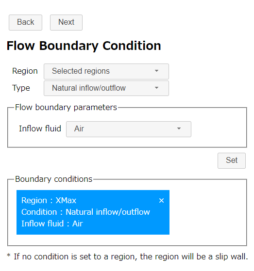
Natural inflow/outflow condition -
Stationary wall boundary
Select "Selected regions" as Region and "Stationary wall" as Type. Then select "XMin", "YMin", "YMax", "ZMin", "ZMax" in navigation view and push .
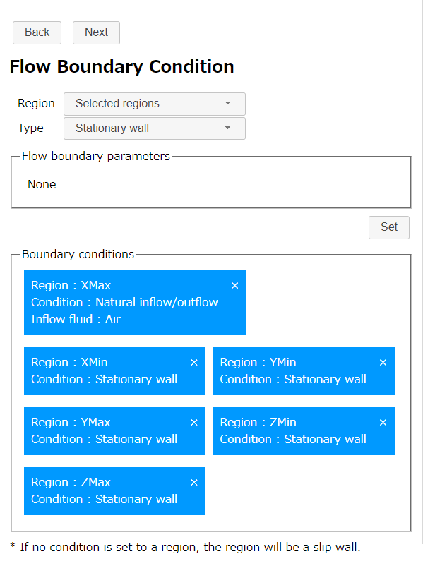
Stationary wall condition
Click button to go to Calculation Settings page.
Calculation Settings
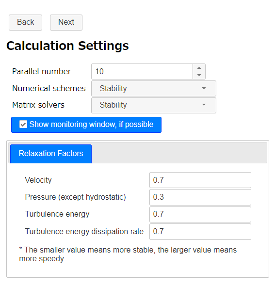
In this section, we set parallel number of CPU core that we use in this calculation (for example, 10).
In this tutorial, we will use a coarse mesh to shorten the calculation time, so we will set both the numerical scheme and the matrix solver to "Stability" since the calculation can be unstable.
Click button to go to Output page.
Output
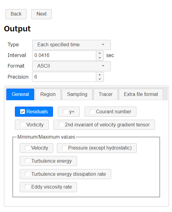
Because this analysis is a transient analysis, select "Each specified time" as Type and enter 0.0416 sec (= about 1/24 sec) to interval.
Click button to go to Export page.
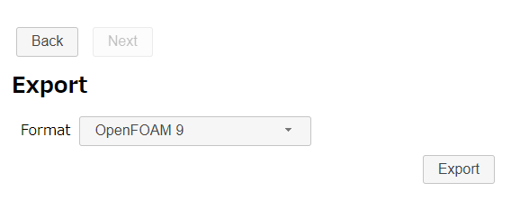
Export
Finally we finished all settings. Click button to export the analysis setting as zipped OpenFOAM case directory "DamBreak.zip". The zip file download starts immediately.
Running a calculation
Extract downloaded file "DamBreak.zip". There is a bash-script "Allrun " in the case directory. So run the script to make mesh and start the OpenFOAM solver by following command.
If the machine that calculation is running has desktop environment and gunuplot was installed, residual convergence chart will be displayed.
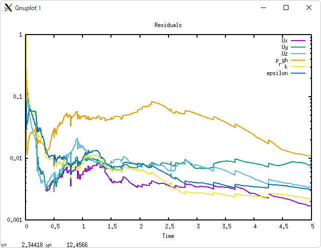
Running in 10 parallel (Inter(R) Core(TM) i7-8700 CPU @ 3.20GHz 3.19GHz), it takes 10 seconds to create a mesh and about 30 minutes to analyze.
Calculation result
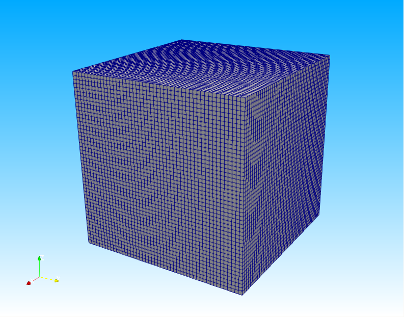
After the calculation, execute a following command to visualize the mesh and the calculation result.
Mesh is as follows.
If we use the Threshold filter of ParaView to visualize the volume ratio (alpha.Water, alpha.Kerosene) with a lower limit of 0.1, we can see the following.