Tutorial : Heat convection by a heater
In this tutorial, we will calculate a heat convection of a room that has a heater and a window facing open air.
Analysis summary
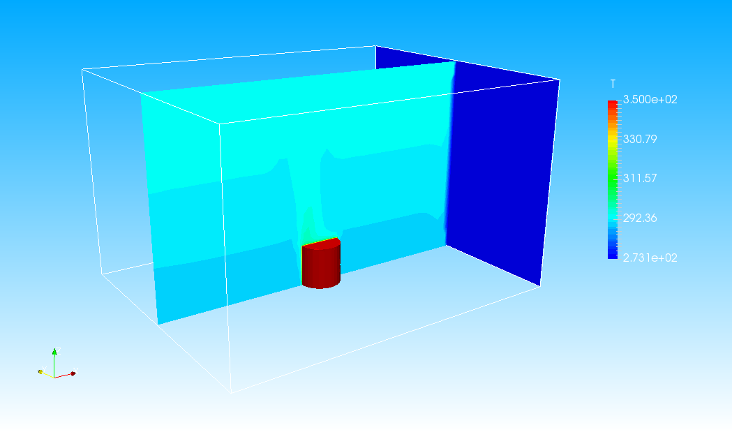
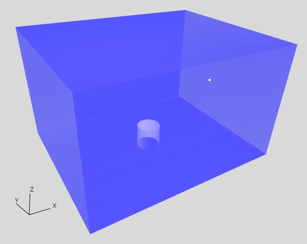
The room has a a window facing open air of 0 °C. And there is a heater of 76.85 °C at the center of a room. We calculate a stationary state of this room and measure the temperatures at wall side and the window side.
Creating an analysis configuration file
Creating a project
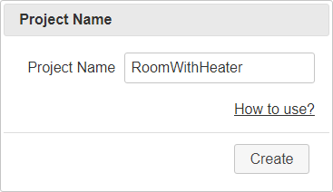
Open XSim. Type "RoomWithHeater" as Project Name and click button to create project.
Importing shapes
We will use prepared shape files in this tutorial. Please download a zipped file from next link, "tutorial-RoomWithHeater.zip", and extract it.
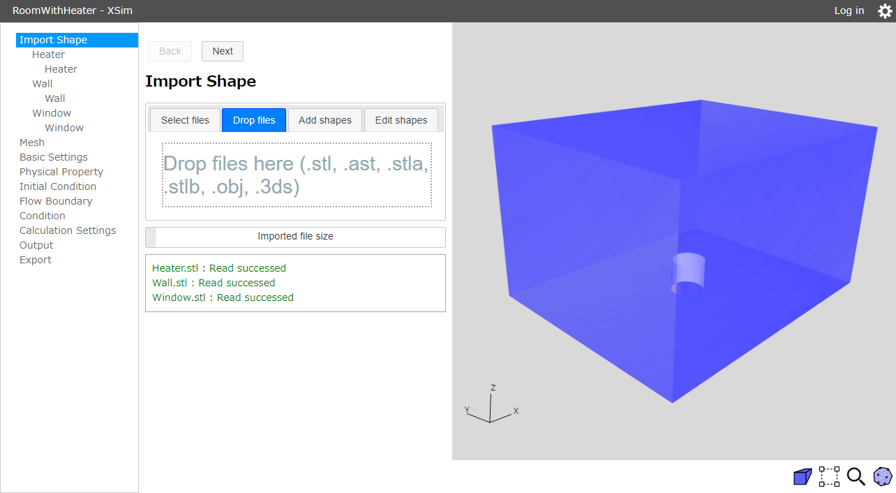
Drag&Drop the extracted file "Wall.stl", "Window.stl" and "Heater.stl" at "Drop files" tab and load it. The loaded shape will be shown in 3D view. You can switch the 3D display to semitransparent by clicking a display-mode button under 3D view.
Click button to go to Mesh page.
Mesh
-
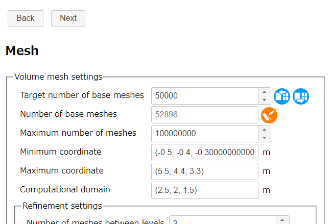
Volume mesh settings
Set 50000 as target number of base meshes. You can preview the base mesh by clicking preview button
 .
.
Setting target number of base meshes 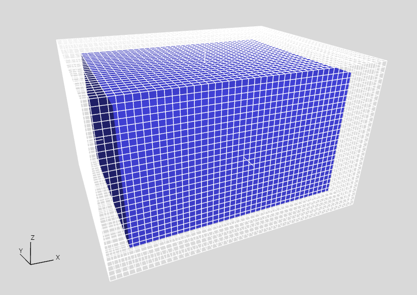
Base mesh preview -
Layer mesh settings
Confirm that 0.3 is set to layer thickness ratio and 3 is set to number of layers. Click "Heater" in Navigation view at left side of the window to select, then click .
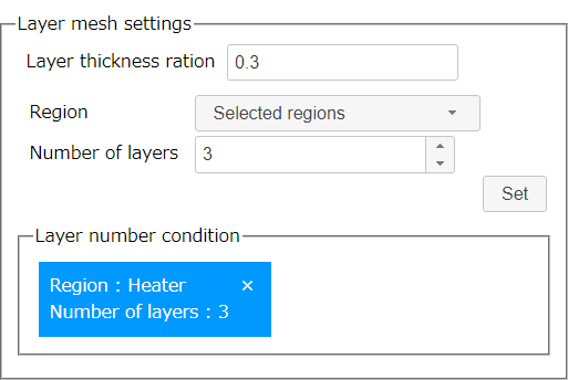
Layer mesh settings
Click button to go to Basic Settings page.
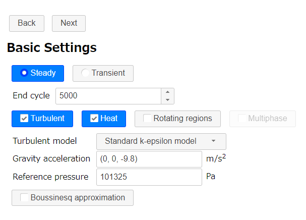
Basic Settings
In this section, we will set a type of analysis. Select "Steady" and set 5000 as end cycle. Then check the .
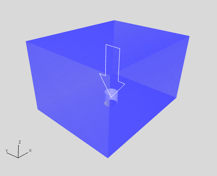
Buoyancy force is taken into account in heat analysis. Therefore a direction of gravity force should be set properly. When is enabled, direction of gravity force will be shown in 3D view.
Click button to go to Physical Property page.
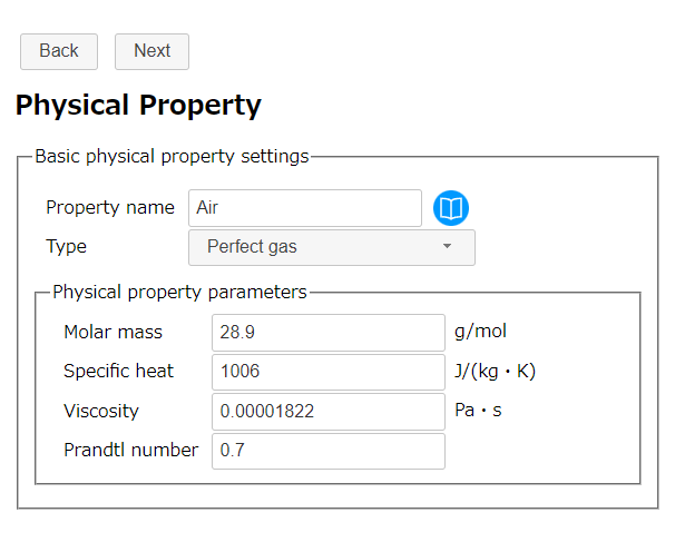
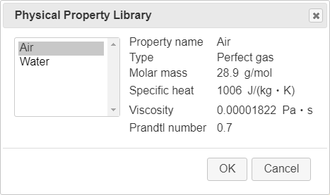
Physical Property
In this section, we will set a type of fluid. Click Physical property library button to show dialog. Select "Air" in the dialog and click .
Click button to go to Initial Condition page.
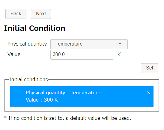
Initial Condition
We will set initial temperature to get final solution as early as possible. Select "Temperature" as physical quantity and set 300 K as value. Then click .
Click button to go to Flow Boundary Condition page.
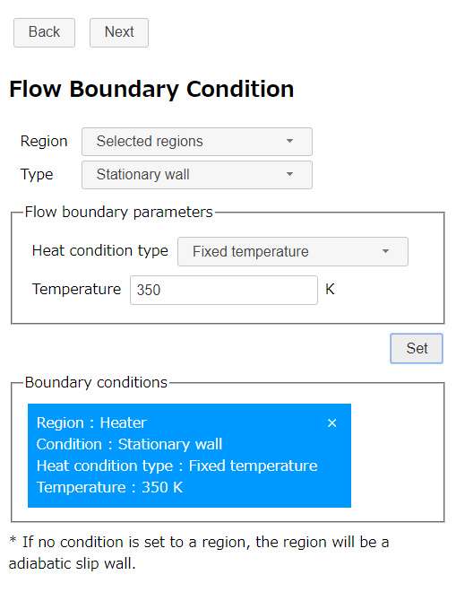
Flow Boundary Condition
-
Heater
Select "Selected regions" as region and "Stationary wall" as type. Then select "Fixed temperature" as heat condition type and set 350 K as temperature. After that, select "Heater" on Navigation view and click .
Fixed temperature condition (Heater) -
Window
Select "Selected regions" as region and "Stationary wall" as type. Then select "Fixed temperature" as heat condition type and set 273.15 K as temperature. After that, select "Window" on Navigation view and click .
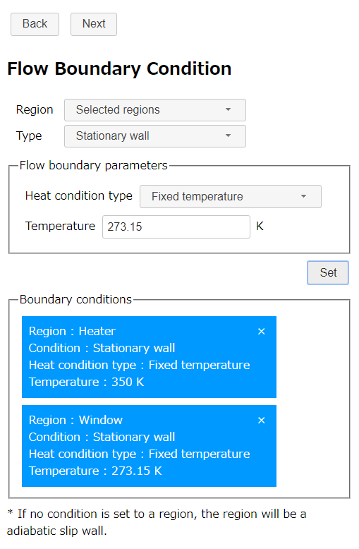
Fixed temperature condition (Window) -
Wall
Select "Selected regions" as region and "Stationary wall" as type. Then select "Adiabatic" as heat condition type. After that, select "Wall" on Navigation view and click .
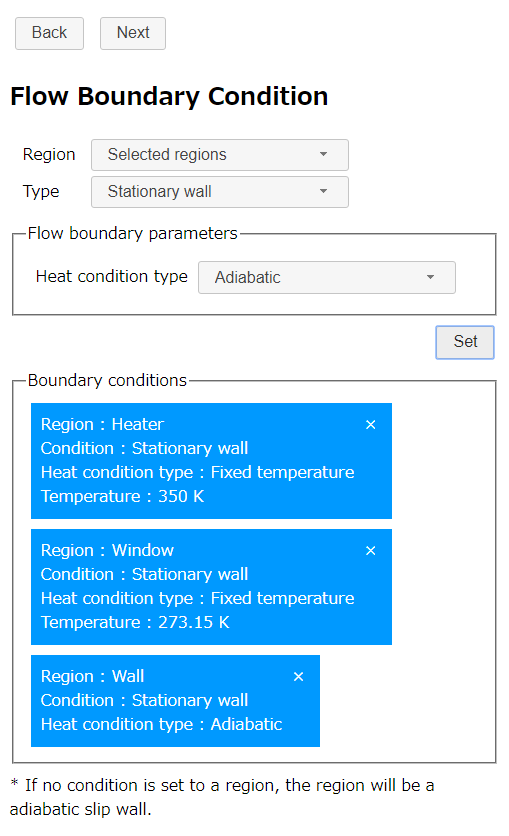
Adiabatic condition (Wall)
Click button to go to Calculation Settings page.
Calculation Settings
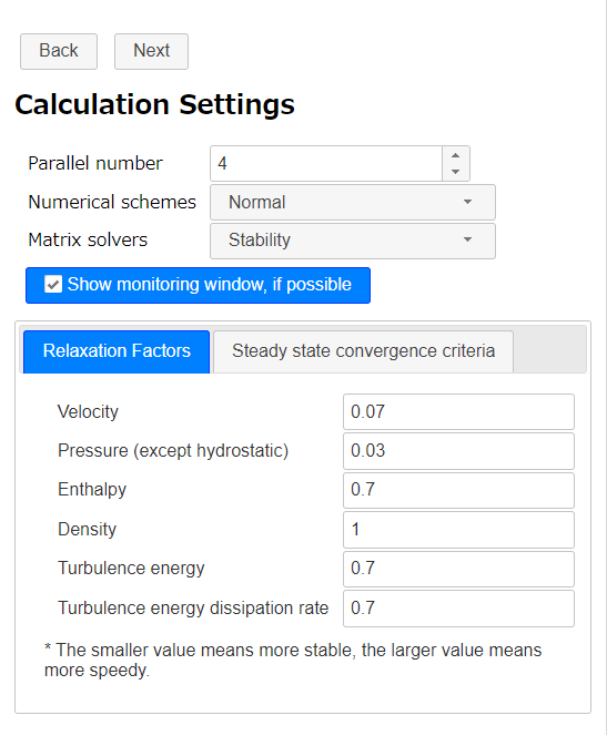
In this section, we set parallel number of CPU core that we use in this calculation (for example, 4).
The calculation of natural convection tend to be instable, so we set relaxation factors for the velocity and pressure to a smaller value of 0.07 and 0.03, respectively, to ensure stable calculations.
Click button to go to Output page.
Output
Because this analysis is a steady analysis, select "Each specified cycles" as type and set 1000 cycles to interval.
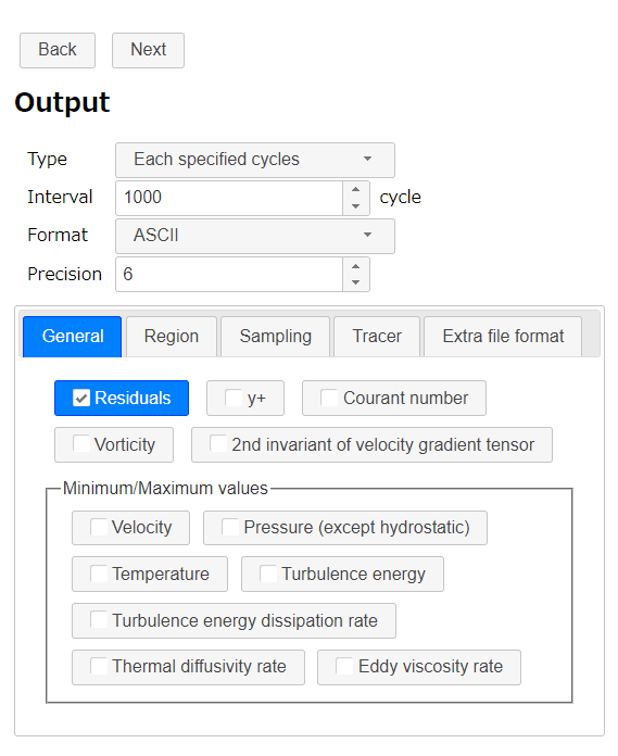
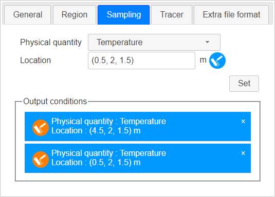
Next, we will make the temperature sampling settings at the specified coordinates.
Select the "Sampling" tab, set "Temperature" as the physical quantity and (4.5, 2, 1.5) as the location, and press . If you push preview button, you can check the sampling position on the 3D view.
With the similar operation, set the temperature at the position (0.5, 2, 1.5) as the sampling target.
Click button to go to Export page.
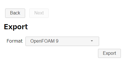
Export
Finally we finished all settings. Click button to export the analysis setting as zipped OpenFOAM case directory "RoomWithHeater.zip". The zip file download starts immediately.
Running a calculation
Extract downloaded file "RoomWithHeater.zip". There is a bash-script "Allrun " in the case directory. So run the script to make mesh and start the OpenFOAM solver by following command.
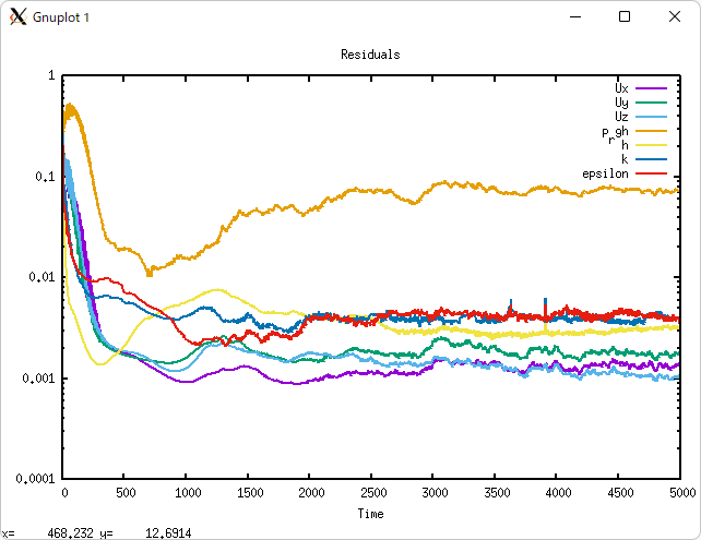
If the machine that calculation is running has desktop environment and gunuplot was installed, residual convergence chart will be displayed.
Running in 4 parallel (Inter(R) Core(TM) i7-8700 CPU @ 3.20GHz 3.19GHz), it takes 1 seconds to create a mesh and about 7 minutes to analyze.
Confirming calculation result
After the calculation, execute a following command to visualize the mesh and the calculation result.
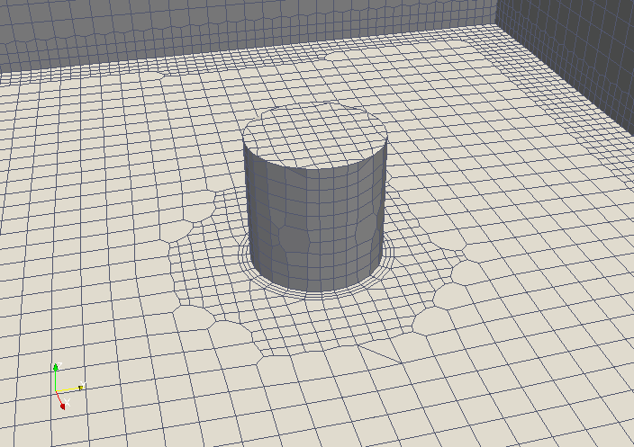
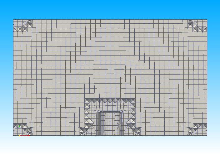
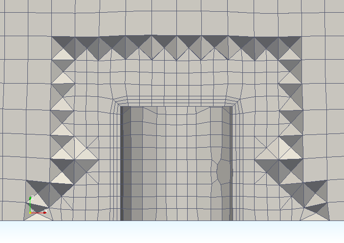
Mesh is as follows.
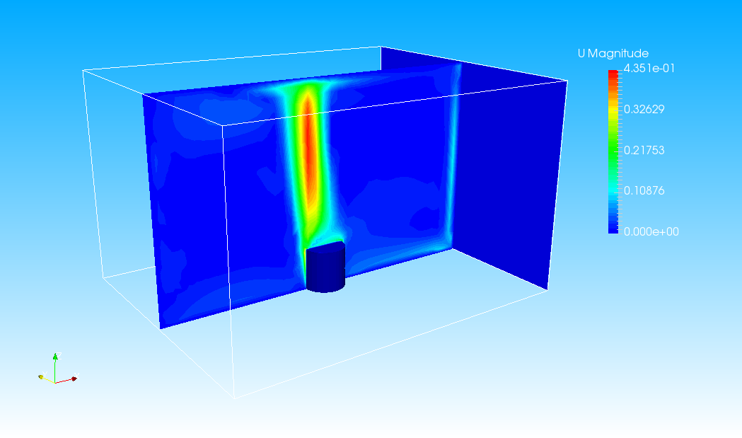
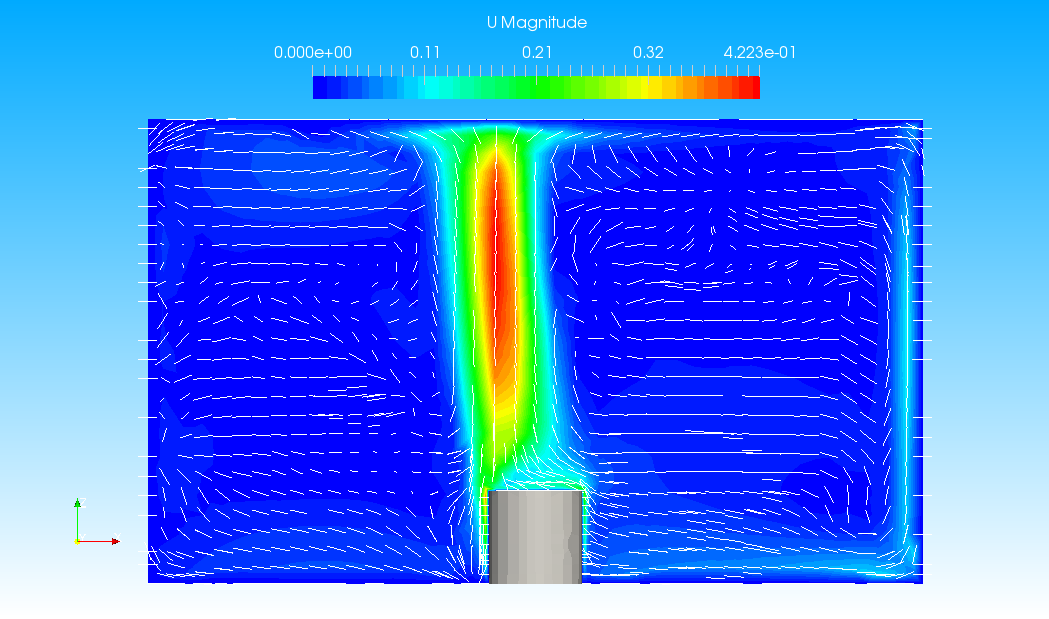
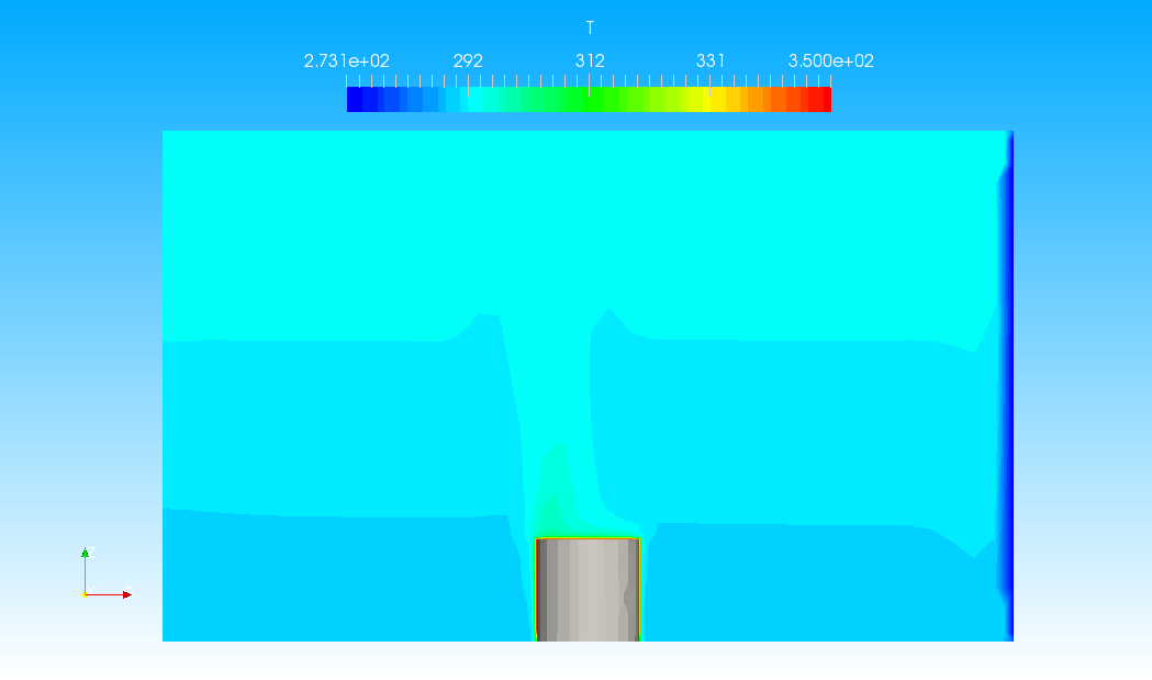
Distributions of Flow velocity and temperature are following.
The sampled temperatures are output at T file in postProcessing/probe(T)/0 folder as following.
# Force coefficients
# Probe 0 (4.5 2 1.5)
# Probe 1 (0.5 2 1.5)
# Time        0             1
0             300           300
1             299.985       300.005
2             299.962       300.005
3             299.964       300.005
…………
4998          287.864       287.883
4999          287.864       287.883
5000          287.864       287.882
The temperature at each sampling position in the final step 1000 is 291.77 K and 291.724 K. It indicates that there is almost no difference in temperature between the wall side and the window side.