Tutorial - Calculation of flow in a sloping channel
In this tutorial, we will calculate flow in a sloping channel with multiphase function.
Analysis summary
We will calculate the water flows through an air-filled, 40 meter long, 11 meter high sloping channel for 20 seconds.
Creating an analysis configuration file
Creating a project
Open XSim. Type "SlopingChannel" as Project Name and click button to create project.
Importing shapes
We will use a prepared shape file in this tutorial. Please download a zipped file from next link, "tutorial-SlopingChannel.zip", and extract it.
Drag&Drop the extracted file "bottom.stl", "inlet.stl", "outlet.stl", "pillar.stl", "sides.stl" and "top.stl" at "Drop files" tab and load it.
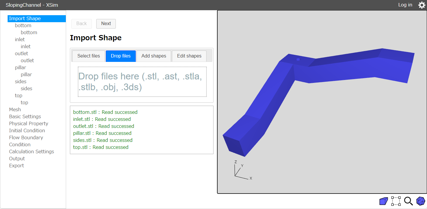
Click button to go to Mesh page.
Mesh
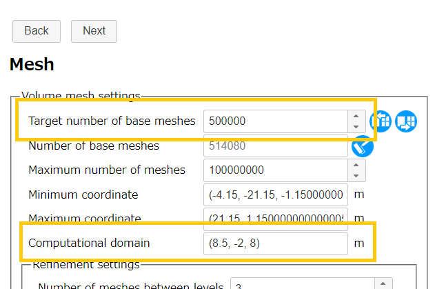
Set 500000 as target number of base meshes. You can preview the base mesh by clicking preview button . And set (8.5, -2, 8) as computational domain to specify the spatial domain for calculation.
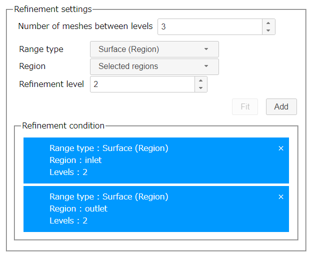
To increase the accuracy of the inflow and outflow, we refine the meshes around the inlet and outlet. Set the Range type to "Surface (Region)", the Region to "Selected regions" and the Refinement level to 2. Select "inlet" and "outlet" in Navigation view on the left side of the window and click .
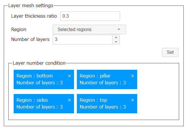
Confirm that 0.3 is set to layer thickness ratio and 3 is set to number of layers. Click "bottom", "pillar", "sides" and "top" in Navigation view to select, then click .
The mesh settings is over. Click button to go to Basic Settings page.
Basic Settings
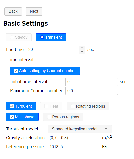
We will set analysis tyoe settings. Select "Transient" and enter "20 sec" as End time. Enter "0.1 sec" as Initial time interval. Then select "Multiphase".
Click button to go to Physical Property page.
Physical Property
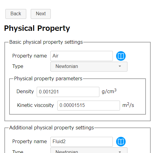
At first, we will set basic physical property.
We want to calculate water flow in the channel filled with air. So we will set air as basic physical property. Push library button at "Basic physical property settings" and select "Air" from the library as basic physical property.
Then we will set "Water" as additional physical properties. Push library button at "Additional physical property settings" and select "Water" from the library. Then push to register the water as additional physical property.
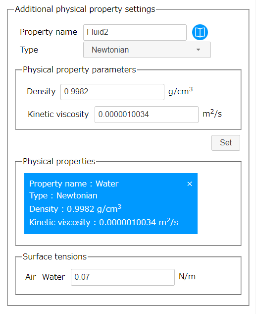
We need to set a surface tension values between each fluid, but for this tutorial we will simplify all of them to "0.07 N/m".
Click button to go to Initial Condition page.
Initial Condition
No configuration is required because we will use default parameters. Click button to go to Flow Boundary Condition page.
Flow Boundary Condition
-
Inflow boundary
Select "Selected regions" as the Region, "Fixed volume flow rate" as the Type, "5 m3/s" as the Volume flow rate, and "Water" as the Inflow fluid, then select "inlet" in the Navigation view and click .
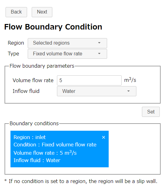
Inflow boundary condition -
Outflow boundary
Select "Selected regions" as the Region, "Fixed static pressure" as the type, "101325 Pa" as the Static pressure, and "Air" as the Inflow fluid, then select "outlet" in the Navigation view and click .
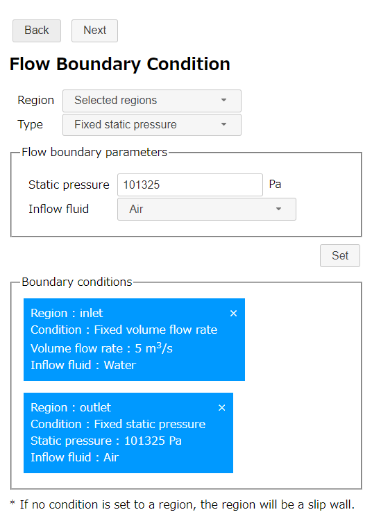
Outflow boundary condition -
Stationary wall boundary
Select "Selected regions" as Region and "Stationary wall" as Type. Then select "bottom", "pillar", "sides", "top" in navigation view and push .
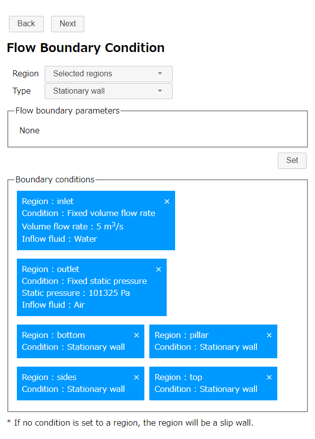
Stationary wall condition
Click button to go to Calculation Settings page.
Calculation Settings
In this section, we set parallel number of CPU core that we use in this calculation (for example, 6).
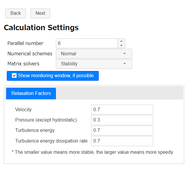
Click button to go to Output page.
Output
Because this analysis is a transient analysis, select "Each specified time" as Type and enter 1 sec to interval.
We also set the output to show the forces acting on the pillar (region "pillar"). In the "Region" tab, select "Selected regions" as the Region, "integral" as the Type, and "Pressure" as the Physical quantity. Select "pillar" in the Navigation view and press .
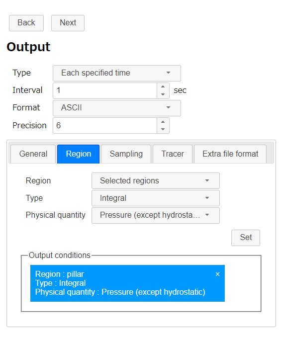
Click button to go to Export page.
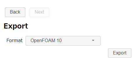
Export
Finally we finished all settings. Click Export button to export the analysis setting as zipped OpenFOAM case directory "SlopingChannel.zip". The zip file download starts immediately.
Running a calculation
Extract downloaded file "SlopingChannel.zip". There is a bash-script "Allrun " in the case directory. So run the script to make mesh and start the OpenFOAM solver by following command.
If the machine that calculation is running has desktop environment and gunuplot was installed, residual convergence chart will be displayed.
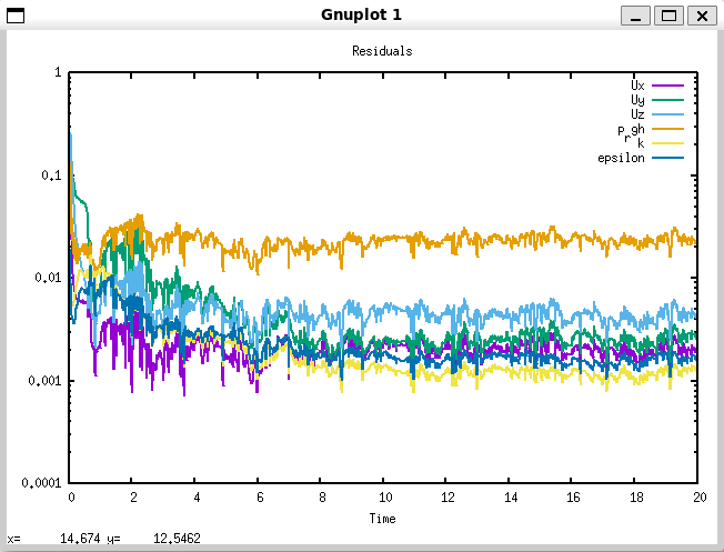
Running in 6 parallel (Inter(R) Core(TM) i7-8700 CPU @ 3.20GHz 3.19GHz), it takes 1 minute to create a mesh and about 40 minutes to analyze.
Calculation result
After the calculation, execute a following command to visualize the mesh and the calculation result.
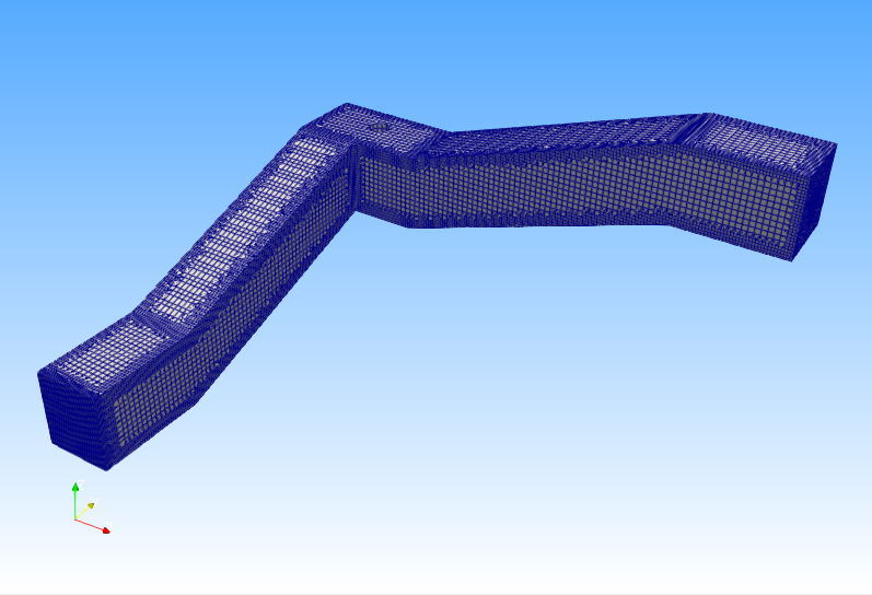
Mesh is as follows.
If we use the Threshold filter of ParaView to visualize the volume ratio (alpha.Water) with a lower limit of 0.1, we can see the following.
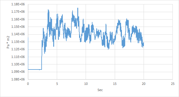
Next, we check the integral values of the pressure at the surface of the pillar. The values are stored under the patchIntegrate(patch=pillar,p_rgh) folder in the postProcessing folder as the file "surfaceFieldValue.dat", which contains the values for each time period as shown below. Note that the reference pressure used in the calculation is 101325 Pa.
# Region type : patch pillar
# Faces  :    182
# Area   :    1.078870e+01
# Time        	areaIntegrate(p_rgh)
0             	1.093165e+06
0.00406504    	1.135852e+06
0.00859202    	1.093317e+06
0.0136245     	1.093210e+06

…………

19.9944       	1.129061e+06
19.9972       	1.128886e+06
20            	1.128877e+06
If we graph this time-series data using Excel or other appropriate software, we can see the following. You can see that the values increase significantly from around 2.3 seconds after the water flow reaches the pillar, and you can also see the maximum and minimum values.