Tutorial - Calculation of inflow/outflow in a tank with a filter
Using porous region feature, We will calculate inflow/outflow and pressure drop in a with a filter.
Analysis summary
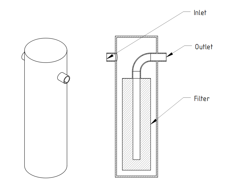
We will calculate steady-state water flow in the tanks with a porous filter. The water flows in at 0.1 m/s from the inlet and flows out from the outlet. We will also calculate the pressure drop (differential pressure between inlet and outlet).
Creating an analysis configuration file
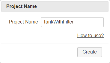
Creating a project
Open XSim. Type "ankWithFilter" as Project Name and click button to create project.
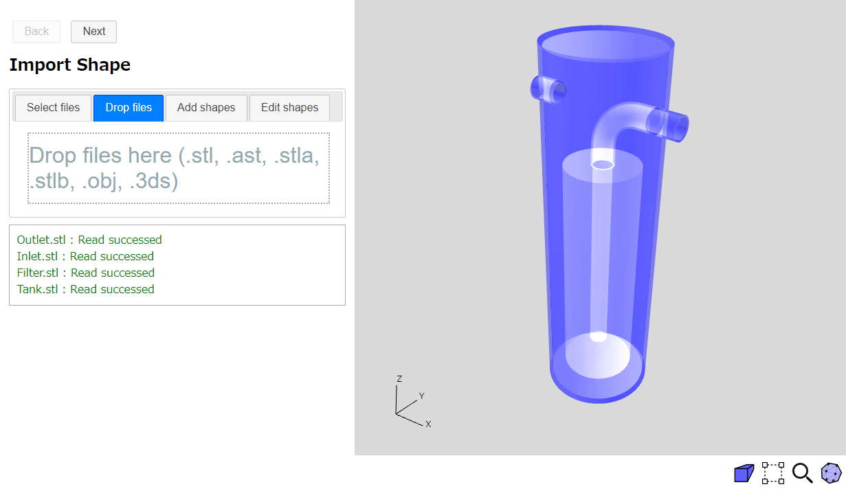
Importing shapes
We will use prepared shape files in this tutorial. Please download a zipped file from next link, "tutorial-TankWithFilter.zip", and extract it.
Drag&Drop the extracted file "Filter.stl", "Tank.stl", "Inlet.stl" and "Outlet.stl" at "Drop files" tab and load it. The loaded shape will be shown in 3D view. You can switch the 3D display to semitransparent by clicking a display-mode button under 3D view.
Click button to go to Mesh page.
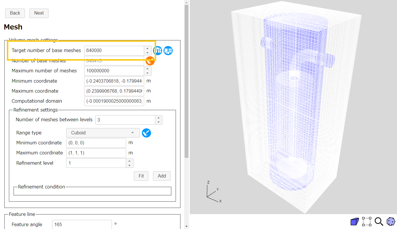
Mesh
Set 640000 as target number of base meshes. You can preview the base mesh by clicking preview button .
.
And we set the number of layers to "3" for the "Tank" region in the layer mesh setting.
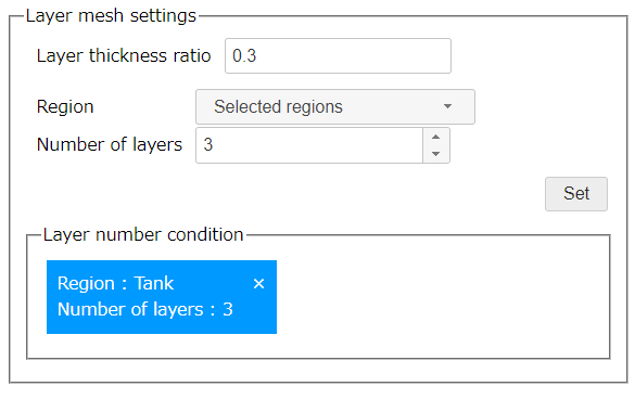
The mesh settings is over. Click button to go to Basic Settings page.
Basic Settings
We set the analysis type. Select "Steady" and set the end cycle to "400". Also select "Porous regions".
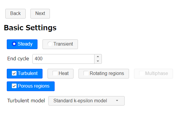
Click button to go to Physical Property page.
Physical Property
No configuration is required because we will use default physical property. Confirm that "Water" is set as the physical property value. Then click button to go to Initial Condition page.
Initial Condition
No configuration is required because we will use default parameters. Click button to go to Flow Boundary Condition page.
Flow Boundary Condition
-
Inlet
Select "Selected regions" as region and "Fixed flow velocity" as type. Then set (0.1, 0, 0) m/s as flow velocity and select "Inlet" on Navigation view. After that, click .
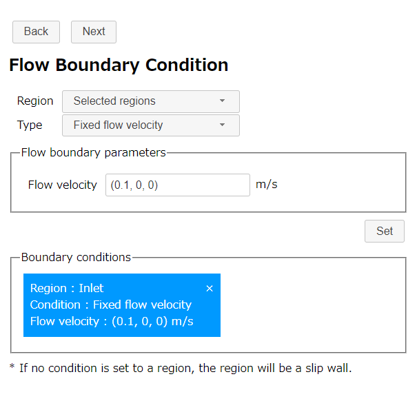
Fixed flow velocity (inlet) -
Outlet
In this calculation, the pressure at "Outlet" will be be used as reference point for pressure. Select "Selected regions" as region and "Fixed static pressure" as type. Then set 0 Pa as static pressure and select "Outlet" on Navigation view. After that, click .
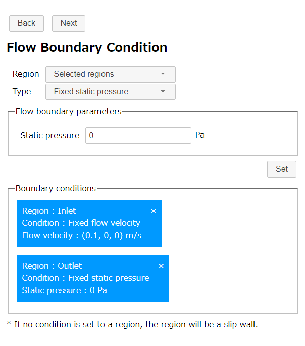
Fixed static pressure (outlet) -
The tank wall
Select "Selected regions" as region and "Stationary wall" as type. Then select "Tank" on Navigation view and click .
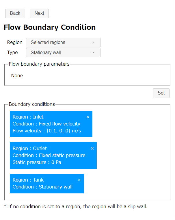
Stationary wall (the tank wall)
After setting the boundary conditions, the 3D view will be as follows.
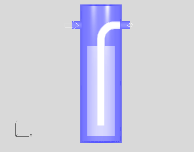
Click button to go to Porous Regions page.
Porous Regions
In this tutorial, We use Darcy-Forchheimer law as the porous model.
Select "Darcy-Forchheimer law" as porous type and "Arbitrary shape (Assembly)" as region type. Then set (5e7, 5e7, 5e7) for d as porous parameter and "Filter" as assembly and press .
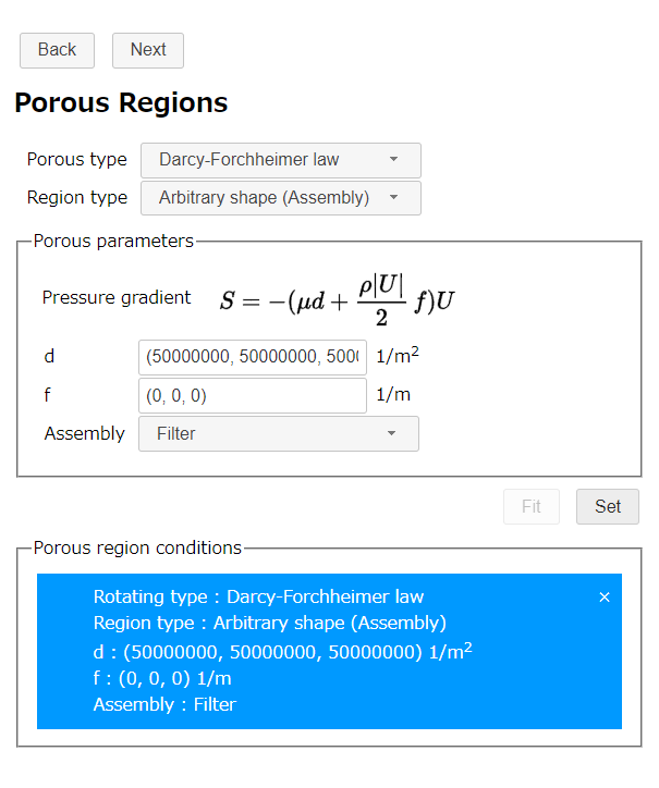
*If you enter "5e7", the value is converted to "50000000 (= 5 x 10⁷)".
Click button to go to Calculation Settings page.
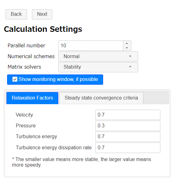
Calculation Settings
In this section, we set parallel number of CPU core that we use in this calculation (for example, 10).
Click button to go to Output page.
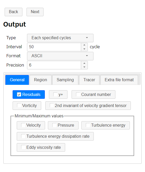
Output
Because this analysis is a steady analysis, select "Each specified cycles" as type and set 50 cycles to interval.
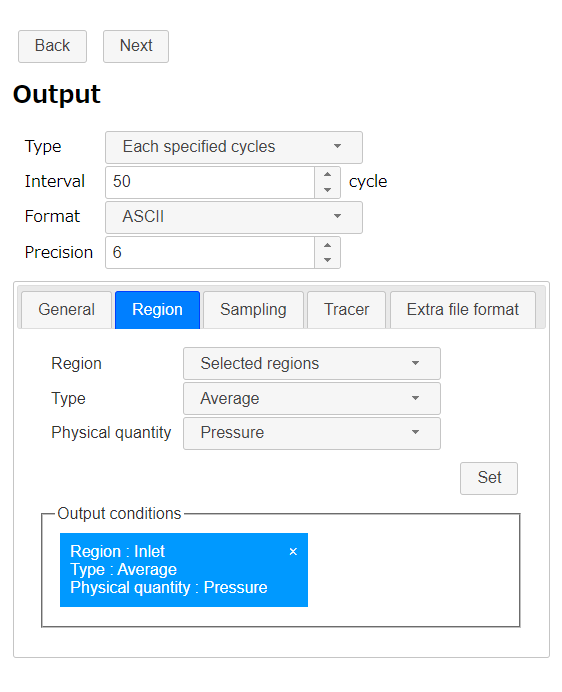
To output inlet pressure with reference to the outlet, select "Region" tab. Select "Selected regions" as region, "Average" as type and "Pressure" as physical quantity. Then select "Inlet" on Navigation view and click .
Click button to go to Export page.
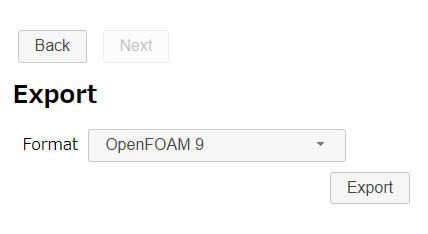
Export
Finally we finished all settings. Click button to export the analysis setting as zipped OpenFOAM case directory "TankWithFilter.zip". The zip file download starts immediately.
Running a calculation
Extract downloaded file "TankWithFilter.zip". There is a bash-script "Allrun " in the case directory. So run the script to make mesh and start the OpenFOAM solver by following command.
If the machine that calculation is running has desktop environment and gunuplot was installed, residual convergence chart will be displayed.
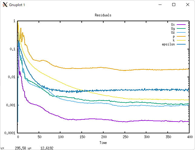
Running in 10 parallel (Inter(R) Core(TM) i7-8700 CPU @ 3.20GHz 3.19GHz), it takes a minute to create a mesh and about 6 minutes to analyze.
Calculation result
After the calculation, execute a following command to visualize the mesh and the calculation result.
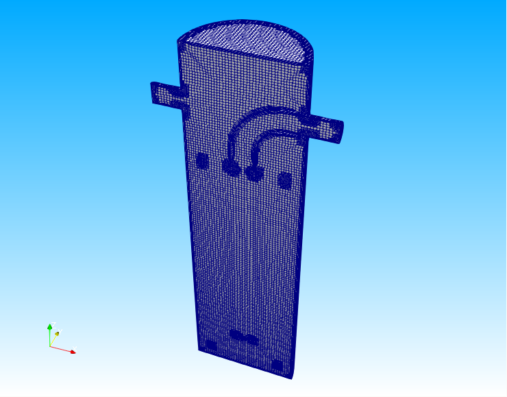
Mesh is as follows.
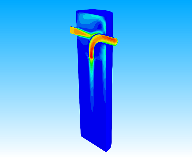
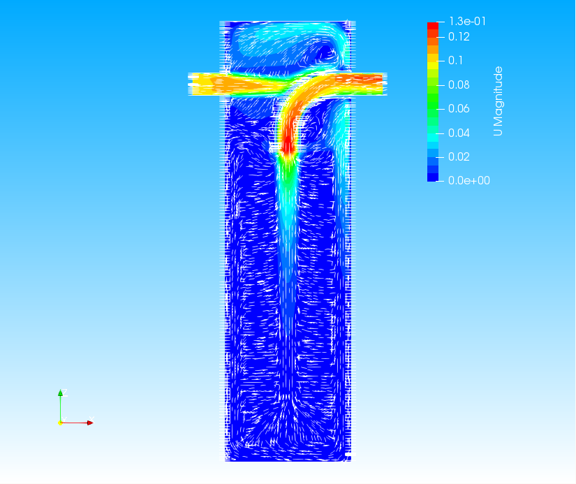
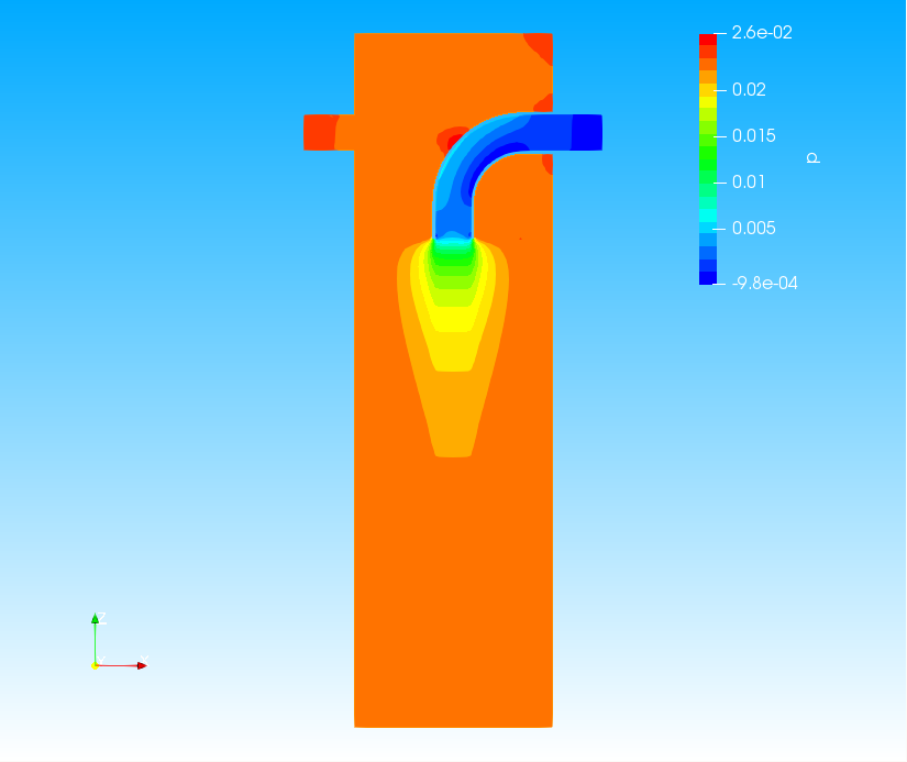
The flow velocity, velocity vector and pressure distribution are also shown below.
Next, check the calculated pressure at the inlet. The average pressure at the inlet is stored in the folder postProcessing/patchAverage(patch=Inlet,p). The output results are as follows.
# Region type : patch Inlet
# Faces  :    299
# Area   :    1.954882e-03
# Time        	areaAverage(p)
0             	0.000000e+00
1             	4.931639e-01
2             	5.779418e-01
3             	2.377576e-01
…………
398           	2.414822e-02
399           	2.414903e-02
400           	2.414786e-02
The first column is the cycles and the second column is the average pressure; The units of pressure are m2/s2, because the fluid is incompressible.